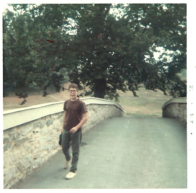

My childhood friend, Carl Hoffman, introduced me to Avalon Hill wargames. Carl is now a history teacher.
It was my good friend, Carl Hoffman, who lived across the street when I was about 10, who introduced me to Avalon Hill (AH) wargames. The AH wargames of the 1960s were perfectly suited to spark a kid’s imagination. The rules were easy to understand (four pages, big type, with illustrations explaining movement and combat), the Combat Results Table (CRT) was straightforward (and taught us to calculate ratios, too), and we could refight Gettysburg or Waterloo on a rainy afternoon. We learned history (Carl became a history teacher) and problem solving (I became a computer scientist). I’m sure many of us had similar experiences forty or fifty years ago.
For a long time I’ve felt that there is a need for similar ‘introductory wargames’ to engage the next generation of grognards and wargamers. While the hardcore aficionados want more complex and detailed games I’ve also understood that we needed simple, introductory games, to entice a new generation. From the beginning, I have always had a simpler wargame embedded inside of General Staff. Specifically, if we remove all the layers of historical simulation, what remains is a simple introductory wargame.
The Layers of Historical Simulation in General Staff
Each layer of historical simulation can be turned on or off when playing a General Staff scenario. The more options you add, the more historically accurate the simulation becomes. The options are:
- Unit strength
- Unit strength is a value from 1 – 4 with units being reduced in steps.
- Unit strength is the actual historic number of troops and every individual casualty is tracked.
- Combat resolution
- Simple Combat Resolution Table like the old AH CRT.
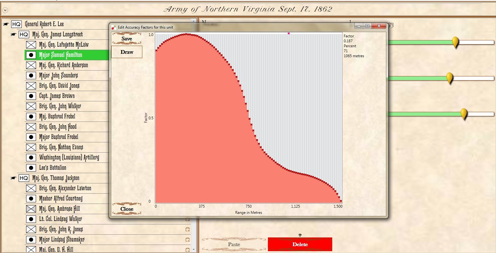
- Complex Combat Resolution Equation taking into effect morale, experience, leadership, terrain, and elevation.
- Moving units
- Units are moved directly by the player.
- Orders to move units are issued down a chain of command from the top HQ to the subordinate HQ via couriers and the rapidity with which the orders are executed depends on the Leadership Value of the subordinate HQ and subordinate units.
- Fog of War (FoW)
- No Fog of War. The entire map is visible and all units (friend and foe) are displayed on it.
- Partial FoW. The entire map is displayed and the sum of what all friendly units can see is displayed.
- Complete FoW. You see only what the commander can see from his HQ and nothing else. All unit positions not directly observable are updated via couriers and are frequently no longer accurate by the time the courier arrives.
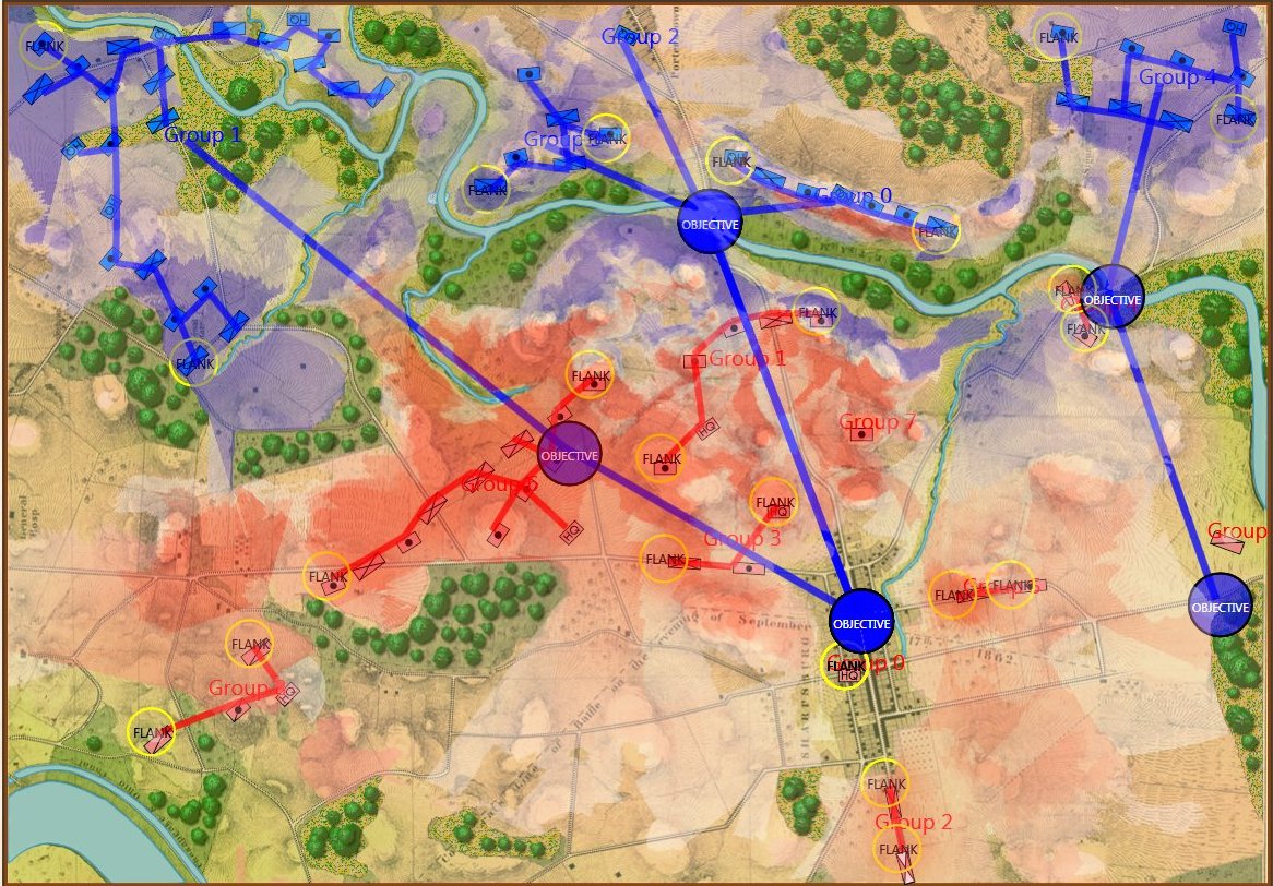
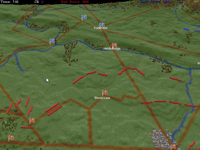
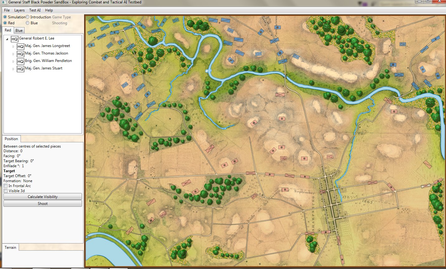
So, at it’s most complex (let’s call this a Historical Accuracy level of 100%) this is what the player commanding the Army of the Potomac (Blue) would see (what General George McClellan could actually see through his telescope on the lawn of the Pry House on the morning of September 17, 1862):
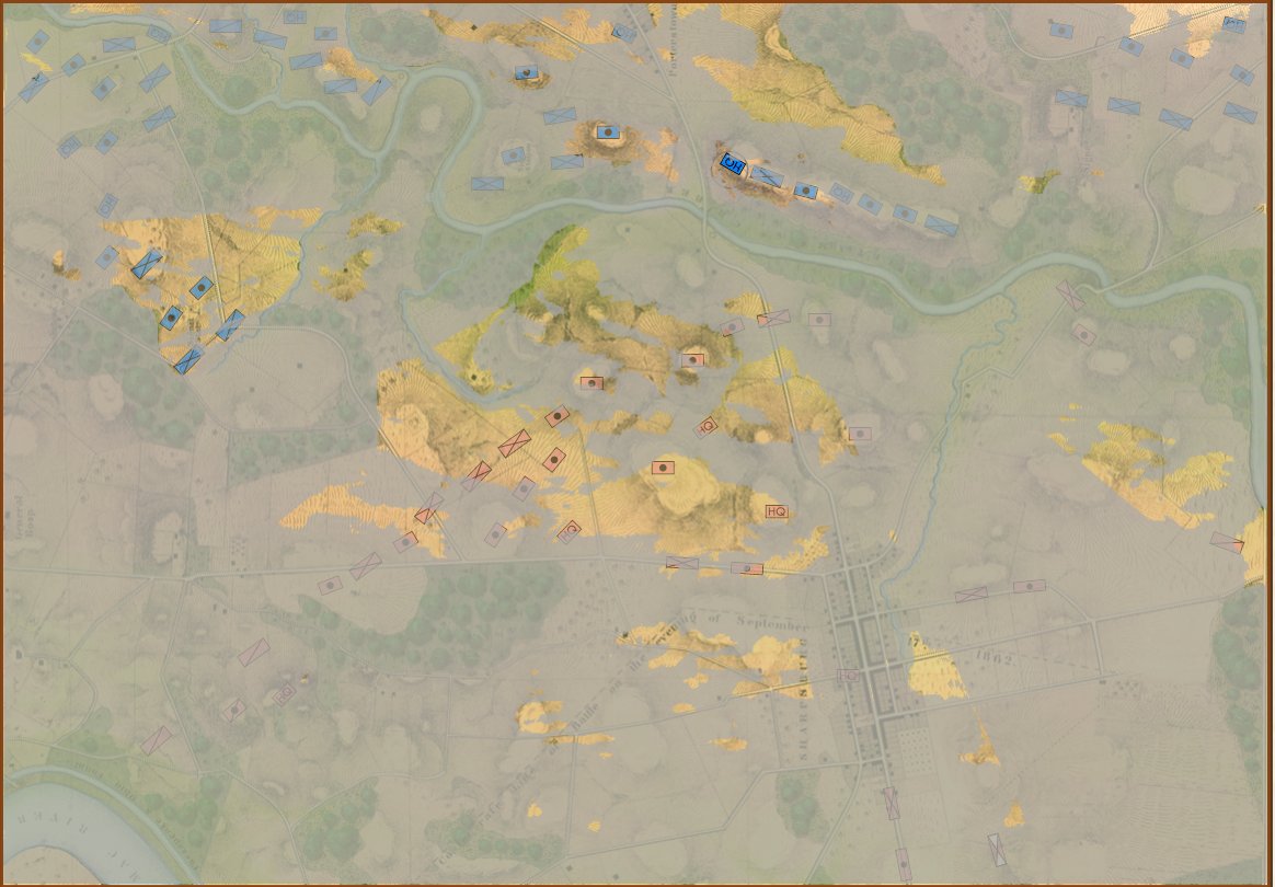
Antietam from the perspective of General George B. McClellan at the Pry House on the east bank of the Antietam Creek. This is complete Fog of War and the highest level of historical accuracy. Screen shot. Click to enlarge.
And, interestingly, this view of what McClellan could see is confirmed in The U. S. Army War College Guide to the Battle of Antietam and The Maryland Campaign of 1862 edited by Jay Luvaas and Harold W. Nelson.”General McClellan and his headquarters staff observed the battle from the lawn of the Pry House… Through a telescope mounted on stakes he enjoyed a panorama view of the fighting… He could see Richardson’s division break through the Confederate position at the Bloody Lane. He could not, however, follow the movements of the First and the Twelfth Corps once they disappeared into the East Woods, which masked the fight for the Cornfield, nor did he witness the attempts to seize Burnside’s bridge to the south because the view from the Pry House was blocked by trees and high ground.” – p. 119.
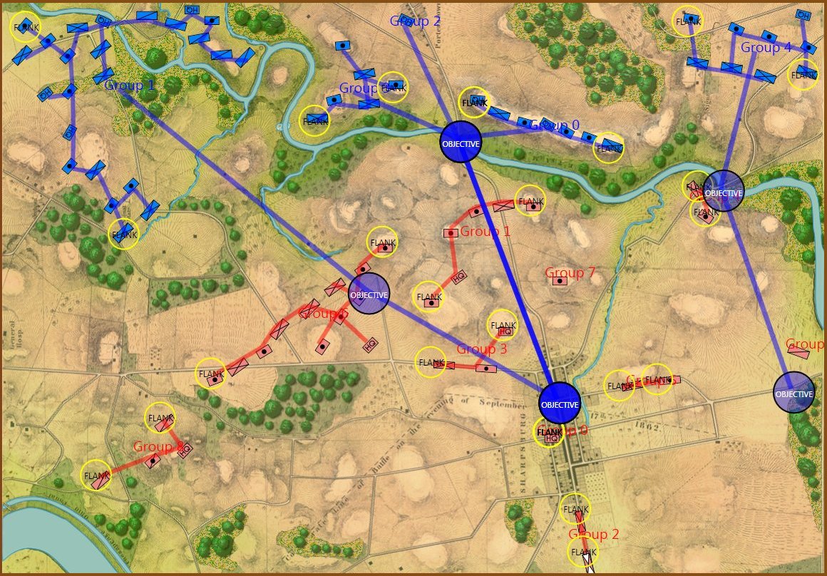
So, the above is the 100% historically accurate view of the battle of Antietam from McClellan’s Headquarters. This is the ‘introductory’ view:
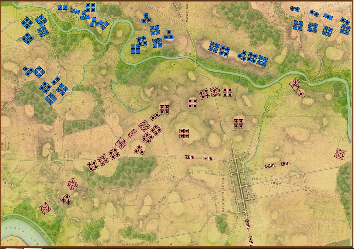
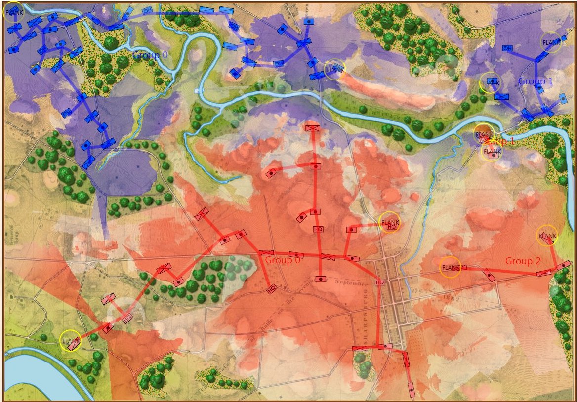
Antietam in ‘Introductory’ mode. Note that unit strengths are represented by one to four icons. Also note the lack of HQs. Screen shot. Click to enlarge.
I first saw the concept of ‘unit steps’ in Jim Dunnigan’s Avalon Hill classic, 1914 and I’m shamelessly using it here. I very much like the simplicity of this system: as units take casualties, they are reduced, in steps, from four icons, to three, to two, etc. I also very much like the idea that this is not an abstraction of the battle of Antietam (or Little Bighorn, or Quate Bras, etc.) but the actual units in their actual locations. This fulfills my requirements for an introductory wargame: historic, teaches tactics and problem solving, easy to play, simple rules, quick to learn and quick to play (I would think a game could easily be played in less than an hour).
Here are some more General Staff scenarios in ‘introductory mode’:
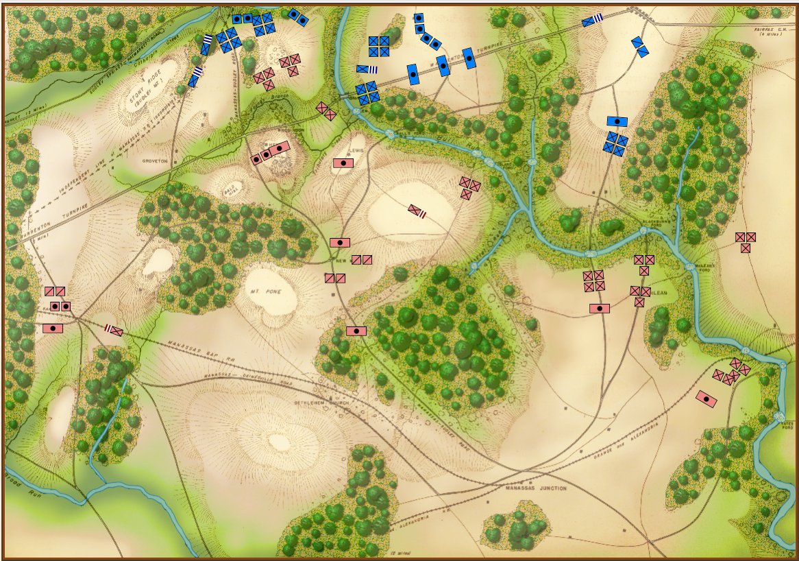
1st Bull Run, 11:30 hours, ‘introductory’ mode. Screen shot. Click to enlarge.
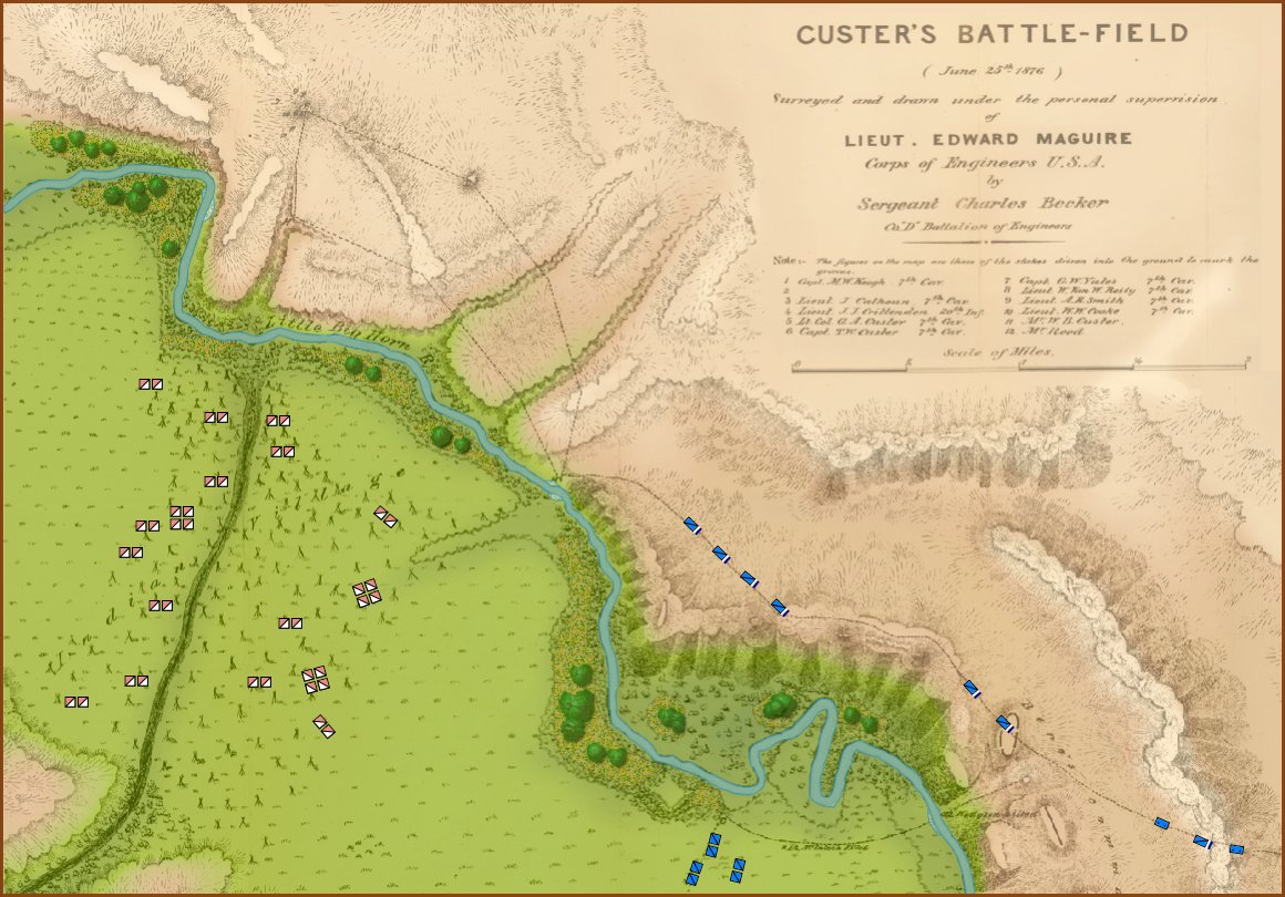
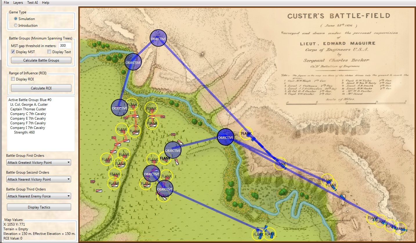
Little Bighorn in ‘introductory’ mode. Screen capture. Click to enlarge.
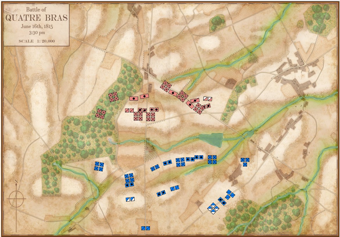
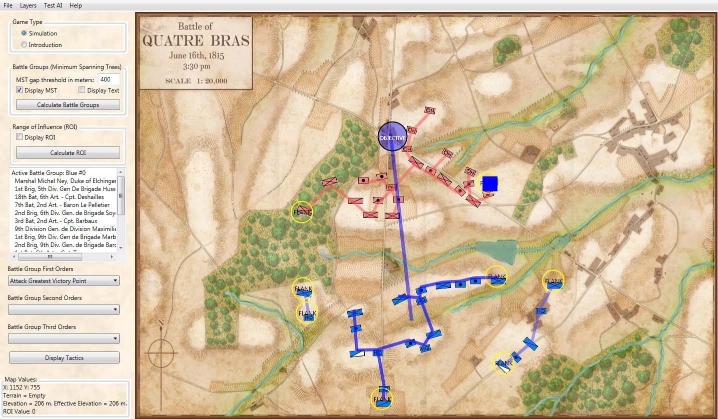
Quatre Bras in ‘introductory’ mode. Screen capture. Click to enlarge.
I could use your help! Announcing a ‘name the mode’ contest!
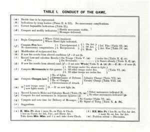
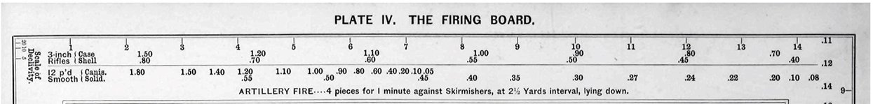
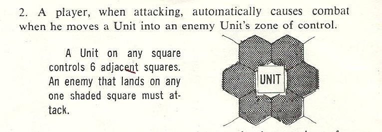
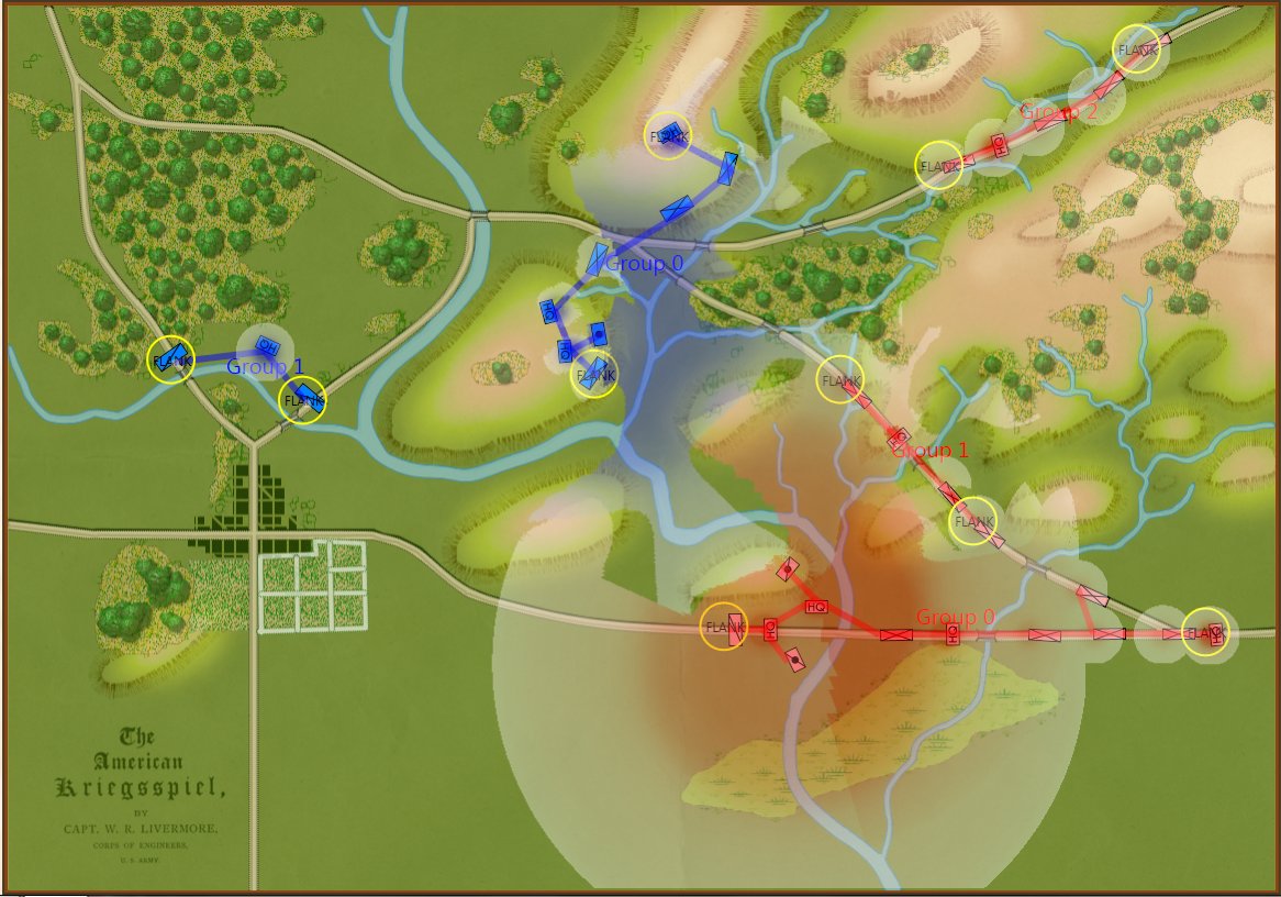
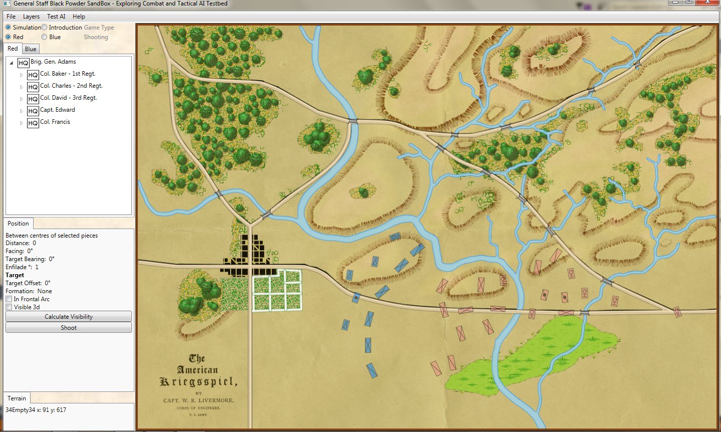
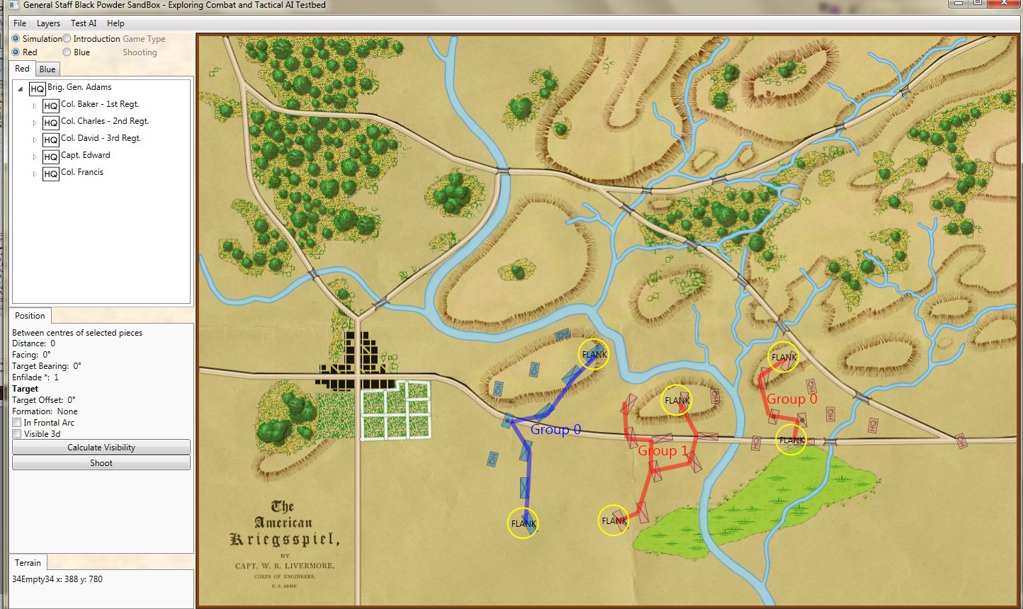
From ‘The American Kriegsspiel. Clicking on this image will take you to the Grogheads.com article on William Livermore’s American Kriegsspiel.
I originally called ‘introductory’ mode, ‘Kriegsspiel’ mode because I was reminded of the maps and blocks that Kriegsspiel uses. However, I pretty quickly received some emails from the Kriegsspiel community complaining – and rightfully so – that Kriegsspiel isn’t an introductory game. Absolutely! And if you’ve ever taken a look at the original rule books and tables you would agree, too.
So, here’s my problem (and how YOU can help): I need a new phrase to replace ‘Kriegsspiel mode’. I’ve been using ‘Introductory mode’ but I just don’t like it. I really need a new name for this version. I’m open to any suggestions. How about a completely made up word? ‘Stratego’ would be great if it hadn’t already been used. So, I’m announcing a contest to ‘name this mode’. The winner will receive 2 General Staff coffee mugs. Please email me (Ezra@RiverviewAI.com) with you suggestions. Thank you for your help!