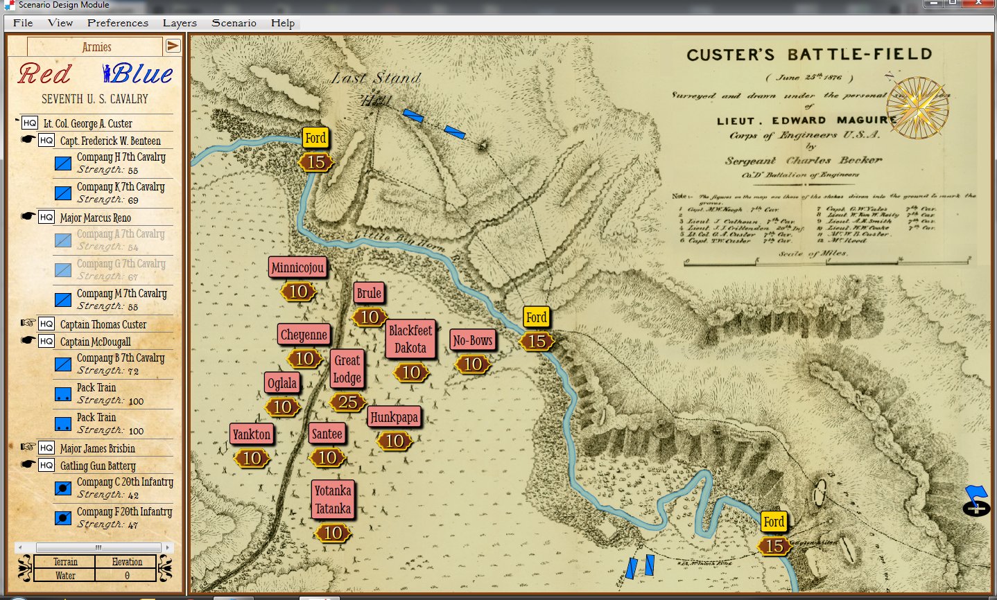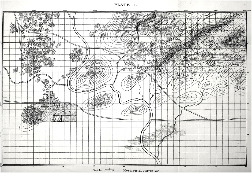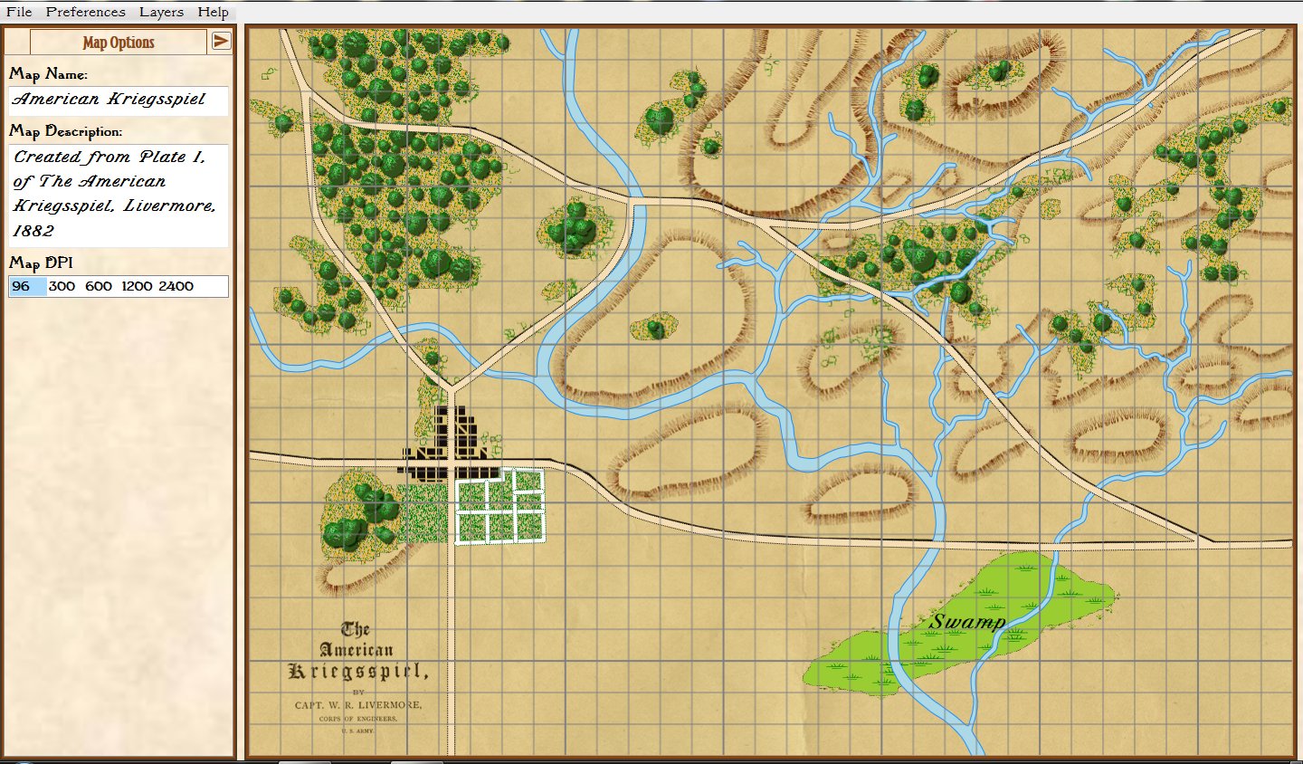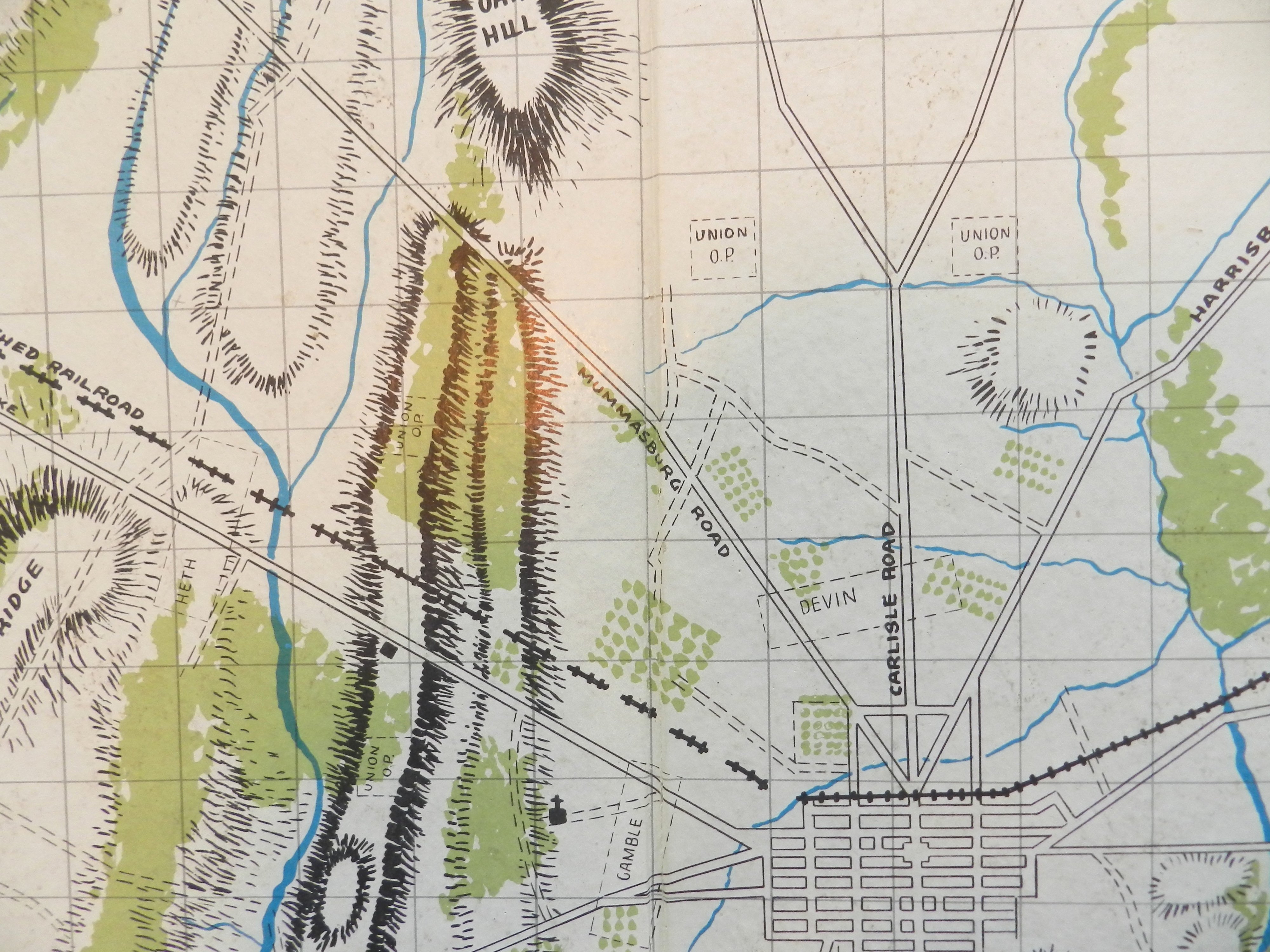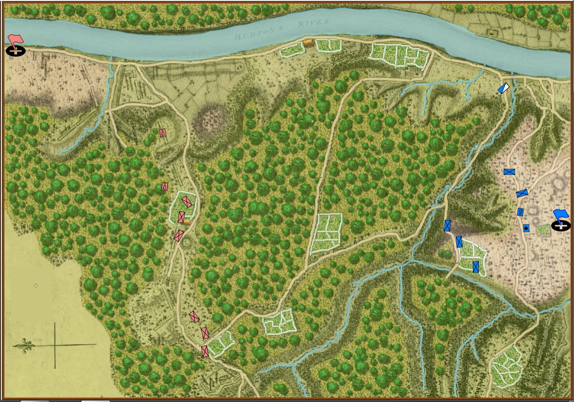
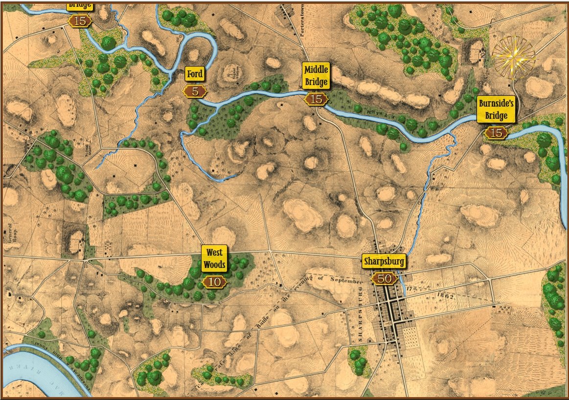
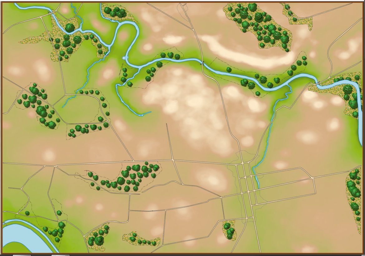
How a map of the battle of Antietam looks to us humans. Screen shot from the General Staff Map Editor. Click to enlarge.
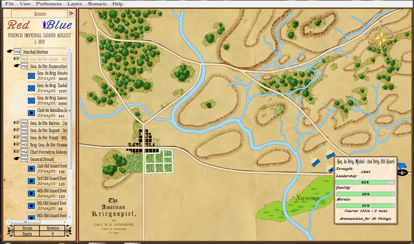
How the computer sees the same map (terrain and elevation). This is actually a screen shot from the Map Editor with the ‘terrain’ and ‘elevation’ layers turned on. Click to enlarge.
Computer vision is the term that we use to describe the process by which a computer ‘sees'1)When describing various AI processes I often use words like ‘see,’ ‘understand,’ and ‘know’ but this should not be taken literally. The last thing I want to do is to get in to a philosophic discussion on computers being sentient. the world in which it operates. Many companies are spending vast sums of money developing driverless or self-driving cars. However, these AI controlled cars have had a number of accidents including four that have resulted in human fatalities.2)https://en.wikipedia.org/wiki/List_of_self-driving_car_fatalities The problem with these systems is not in the AI – anybody who has played a game with simulated traffic (LA Noir, Grand Theft Auto, etc.) knows that. Instead, the problem is with the ‘computer vision’; the system that describes the ‘world view’ in which the AI operates. In one fatality, for example, the computer vision failed to distinguish a white semi tractor trailer from the sky.3)https://www.theguardian.com/technology/2016/jun/30/tesla-autopilot-death-self-driving-car-elon-musk Consequently, the AI did not ‘know’ there was a semi directly in front of it.
In my doctoral research I created a system by which a program could ‘read’ and ‘understand’ a battlefield map4)TIGER: An Unsupervised Machine Learning Tactical Inference Generator http://www.riverviewai.com/download/SidranThesis.html. This is the system that we use in General Staff.
The two images, above, show the difference in how a human commander and a computer ‘see’ the same battlefield. In the top image the woods, the hills and the roads are all obvious to us humans.
The bottom, or ‘computer vision’ image, is a bit of a cheat because this is how the computer information is visually displayed to the human designer in the General Staff Map Editor. The bottom image is created from four map layers (any of which can be displayed or turned off):
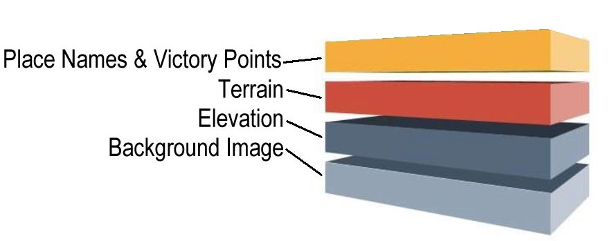
The four layers that make up a General Staff map.
The background image layer in a General Staff map is the beautiful artwork shown in the top image. The place names and Victory Points layer are also displayed in the top image. The terrain and elevation layers are described below:
The next three images are actual visual representations of the contents of memory where these terrain values are stored (this is built in to the General Staff Map Editor as a debugging tool):
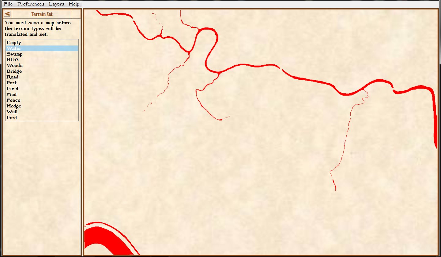
Screen shot from the Map Editor showing just terrain labeled as ‘water’. Click to enlarge
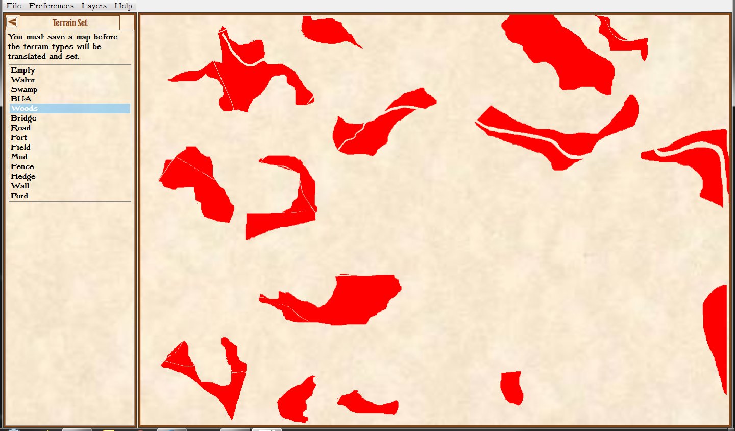
Screen shot from the General Staff Map Editor showing the terrain labeled as ‘woods’. Click to enlarge.
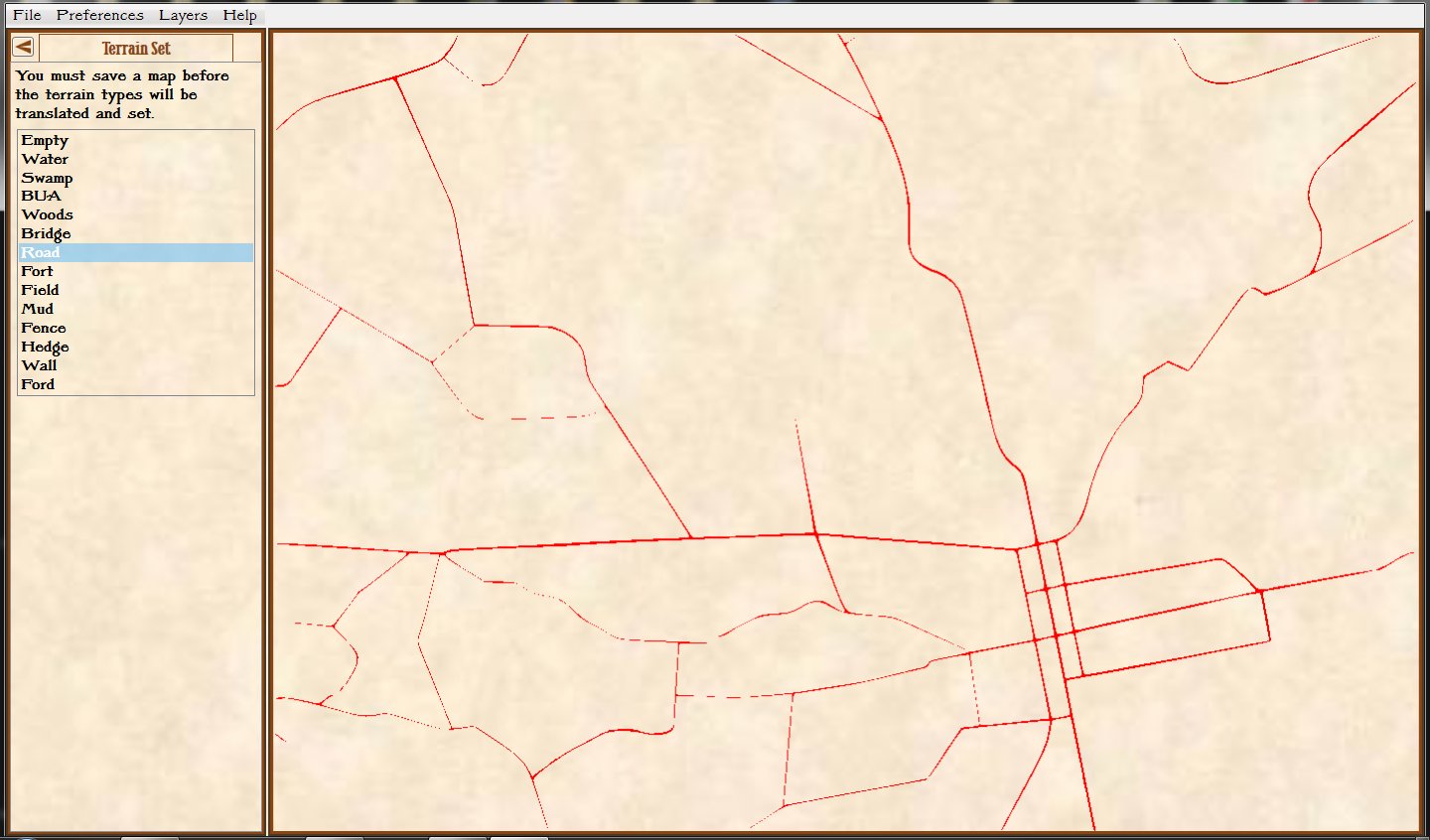
Screen shot from the General Staff Map Editor showing the terrain labeled ‘road’. Click to enlarge.
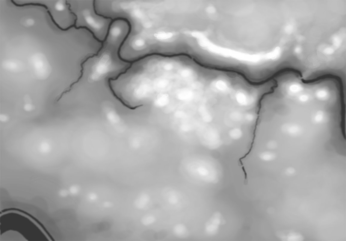
A heightmap for Antietam. This is a visual representation of elevation in meters (darker = lower, lighter = higher). Click to enlarge.
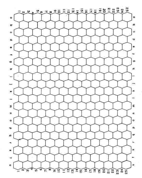
 To computers, an image is a two-dimensional array; like a giant tic-tac-toe or chess board. Every square (or cell) in that board contains a value called the RGB (Red, Green, Blue5)Except in France where it’s RVB for Rouge, Vert, Bleu ) value. Colors are described by their RGB value (white, for example, is 255,255,255). If you find this interesting, here is a link to an interactive RGB chart. General Staff uses a similar system except instead of the RGB system each cell contains a value that represents various terrain types (road, forest, swamp, etc.) and another, identical, two-dimensional array, contains values that represent the elevation in meters. To make matters just a little bit more confusing, computer arrays are actually not two-dimensional (or three-dimensional or n-dimensional) but rather a contiguous block of memory addresses. So, the terrain and elevation arrays in General Staff which appear to be two-dimensional arrays of 1155 x 805 cells are actually just 929,775 bytes long hunks of contiguous memory. To put things in perspective, just those two arrays consume more RAM than was available for everything in the original computer systems (Apple //e, Apple IIGS, Atari ST, MS DOS, Macintosh and Amiga) that I originally wrote UMS for.
 So, not surprisingly, a computer stores its map of the world in which it operates as a series of numbers 6)Yes, at the lowest level the numbers are just 1s and 0s but we’ll cover that before the midterm exams. that represent terrain and elevation. But, how does a human commander read a map? I posed this question to Ben Davis, a neuroscientist and wargamer, and he suggested looking at a couple of studies. In one article7)https://www.citylab.com/design/2014/11/how-to-make-a-better-map-according-to-science/382898/, Amy Lobben, head of the Department of Geography at the University of Oregon, said, “…some people process spatial information egocentrically, meaning they understand their environment as it relates to them from a given perspective. Others navigate more allocentrically, meaning they look at how other objects in the environment relate to each other, regardless of their perspective. These preferences are linked to different regions of the brain.” Another8)https://www.researchgate.net/publication/251187268_USING_fMRI_IN_CARTOGRAPHIC_RESEARCH reports the results of fMRI scans while, “subjects perform[ed] navigational map tasks on a computer and again while they were being scanned in a magnetic resonance imaging machine.” to identify specific, “involvement or non-involvement of the brain area.. doing the task.”
So, how computers and human commanders read and process maps is quite different. But, at the end of the day, computers are just manipulating numbers following a series of algorithms. I have written extensively about the algorithms that I have developed including:
- “Algorithms for Generating Attribute Values for the Classification of Tactical Situations.”
- “Implementing the Five Canonical Offensive Maneuvers in a CGF Environment.”
- “Good Decisions Under Fire: Human-Level Strategic and Tactical Artificial Intelligence in Real-World Three-Dimensional Environments.”
- “Current Methods to Create Human-Level Artificial Intelligence in Computer Simulations and Wargames”
- Human Level Artificial Intelligence for Computer Simulations and Wargames.
- An Analysis of Dimdal’s (ex-Jonsson’s) ‘An Optimal Pathfinder for Vehicles in Real-World Terrain Maps’
These papers, and others, can be freely downloaded from my web site here.
As always, please feel free to contact me directly if you have any questions or comments.
References
| ↑1 | When describing various AI processes I often use words like ‘see,’ ‘understand,’ and ‘know’ but this should not be taken literally. The last thing I want to do is to get in to a philosophic discussion on computers being sentient. |
|---|---|
| ↑2 | https://en.wikipedia.org/wiki/List_of_self-driving_car_fatalities |
| ↑3 | https://www.theguardian.com/technology/2016/jun/30/tesla-autopilot-death-self-driving-car-elon-musk |
| ↑4 | TIGER: An Unsupervised Machine Learning Tactical Inference Generator http://www.riverviewai.com/download/SidranThesis.html |
| ↑5 | Except in France where it’s RVB for Rouge, Vert, Bleu |
| ↑6 | Yes, at the lowest level the numbers are just 1s and 0s but we’ll cover that before the midterm exams. |
| ↑7 | https://www.citylab.com/design/2014/11/how-to-make-a-better-map-according-to-science/382898/ |
| ↑8 | https://www.researchgate.net/publication/251187268_USING_fMRI_IN_CARTOGRAPHIC_RESEARCH |