Category Archives: Artificial Intelligence

Battle Lines, Commanders & Computers

When we look at maps of battles even the novice armchair general can quickly trace the battle lines of the armies. Recognizing battle lines is one of the most important skills a commander – or a wargaming Artificial Intelligence (AI) – can possess. Without this ability how will you identify the flanking units? And if you can’t identify the units at the end of a line, how will you implement a flanking attack around them? Equally important is the ability to identify weak points in a battle line.

The algorithm for detecting battle lines and flank units is one of the ‘building block’ algorithms of my TIGER / MATE tactical AI and first appeared in my paper, Implementing the Five Canonical Offensive Maneuvers in a CGI Environment1)http://riverviewai.com/papers/ImplementingManeuvers.pdf. I will discuss how the algorithm works at the end of this blog. For now, just accept that it finds lines and flanks.

Let’s look at some examples of the General Staff AI ‘parsing’ unit positions. First, the battle of Antietam, situation at dawn (by the way, Antietam is one of the free scenarios included with the General Staff Wargaming System):

The battle of Antietam, dawn, September 17, 1863. Screen shot from the General Staff Sand Box program. Click to enlarge.

This is how a human sees the tactical situation: units on a topographical map. But, the computer AI sees it quite differently. In the next image, below, the battle lines and elevation are displayed as the AI sees the battle (note: the AI also ‘sees’ the terrain but, for clarity, that is not being shown in this screen capture):

The battle of Antietam, September 17, 1862 dawn, with computer AI battle lines and elevation displayed. Note: the identification of flank units. Both red and blue forces are assembling on the field. Click to enlarge.

What is immediately obvious is that Red (Confederate) forces are hastily constructing a battle line while Blue (Union) forces are beginning to pour onto the battlefield to attack.  Let us now ask the question: what is the weakest point of the Red battle line? Where should Blue attack? This point is sometimes called the Schwerpunkt. German for point of maximum effort2)See also, “Clausewitz’s Schwerpunkt Mistranslated from German, Misunderstood in English” Military Review, 2007 https://www.armyupress.army.mil/Portals/7/military-review/Archives/English/MilitaryReview_20070228_art014.pdf. Where should Blue concentrate its forces?

Computer AI representation of battle lines for Antietam, dawn September 17, 1862. The AI is locating the Schwerpunkt or place to attack. Click to enlarge.

Now that the weakest points of Red’s battle line have been identified, Blue (assuming Blue is being controlled by the AI) can exploit it by attacking the gaps in Red’s battle line. The Blue AI can order either a Penetration or Infiltration Maneuver to exploit these gaps (the following images are from my paper, “Implementing the Five Canonical Offensive Maneuvers in a CGF Environment.” Note, in the TIGER / MATE screen shots below Range of Influence (ROI) is also visible:

From the paper, “Implementing the Five Canonical Offensive Maneuvers.”

Both of these maneuvers are possible because the AI has identified weak points in the OPFOR (Opponent Forces) battle lines. Equally important when discussing battle lines are the location of the flanks. The next two images use the original American Kriegsspiel (1882) map which is also included in the General Staff Wargaming System:

The original American Kriegsspiel map (1882) restored and now used in the General Staff Wargaming System. Screen shot from the General Staff Sand Box AI test program. Click to enlarge.

In this screen capture from the General Staff Wargaming System Sand Box AI test program battle lines are displayed by the AI. Note the flank units and especially the unanchored (or open) Blue flank. Click to enlarge.

Identifying flank units is vitally important in the Turning Maneuver and the Envelopment Maneuver:

Knowing the location of flank units is also important for classifying tactical positions (this will be the subject of an upcoming blog).

So, how does this algorithm work?

I’ve never been a fan of graph theory; or heavy mathematical lifting in general. One of the required classes in grad school was Design and Analysis of Algorithms and it got into graph theory quite a bit. The whole time I was thinking, “I’m never going to use any of this stuff, but I have to get at least a B+ to graduate,” so I took a lot of notes and studied hard. Later, when I was looking for a framework to understand tactics and to write a tactical AI it became obvious that graph theory was at least part of the solution. Maps are routinely divided into a grid, unit locations can be points (or vertices) at the intersections of these lines. Battle lines can be edges that connect the vertices. I need to publicly thank my doctoral advisor, Dr. Alberto Segre, for first suggesting that battle lines could be described using something called a Minimum Spanning Tree3)https://en.wikipedia.org/wiki/Minimum_spanning_tree (MST). An MST is the minimum possible distances (edge weights to be precise) to connect all the vertices in a tree (or a group, as I call them in the above screen shots).

I ended up implementing Kruskal’s algorithm4)https://en.wikipedia.org/wiki/Kruskal’s_algorithm for identifying battle lines. It is what is called a ‘greedy algorithm’ and it runs in O(E log V) which means it gets slower as we add more units but we’re never dealing with gigantic numbers of individual units in an Order of Battle (probably around 50 is the maximum) so it takes less than a second to calculate and display battle lines for both Red and Blue.

Lastly, and I guess this is my contribution to military graph theory, I realized that the flank units of any battle line must be the maximally separated units. That is to say, that the two units in a battle line that are the farthest apart are the flank units.

Obviously, this is a subject that I find fascinating so please feel free to contact me directly if you have any questions or comments.


Computational Military Reasoning Part 4: Learning

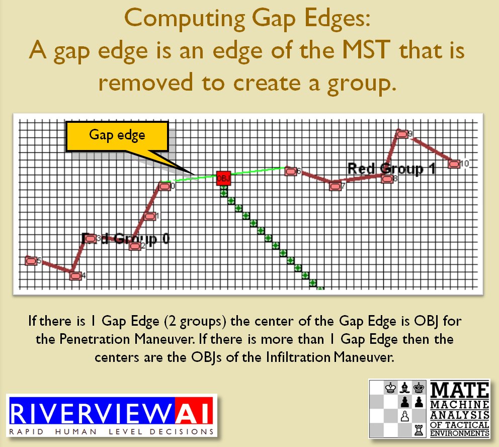
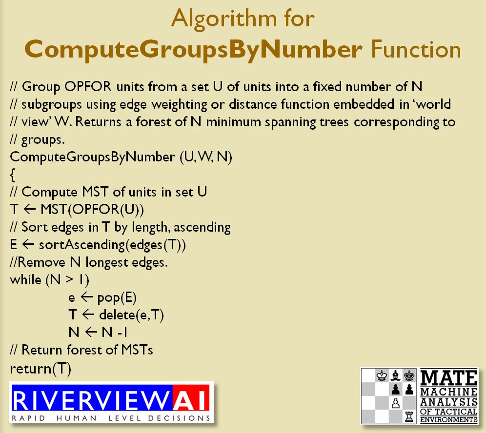
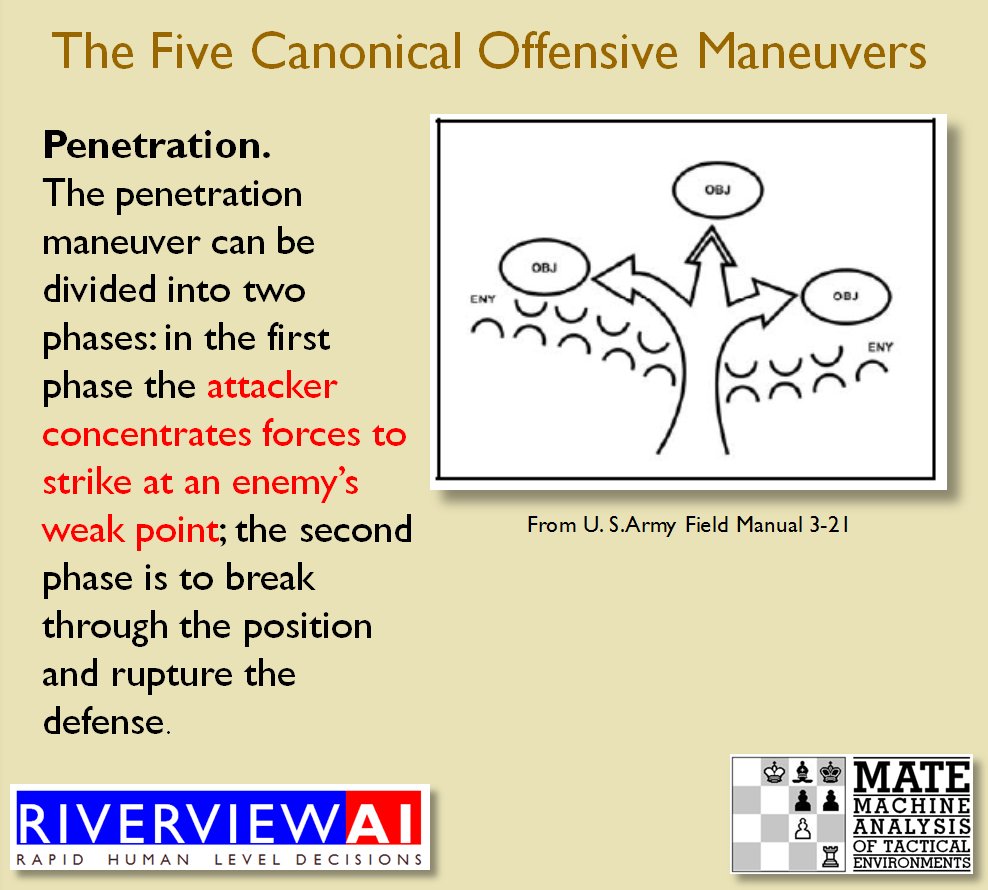
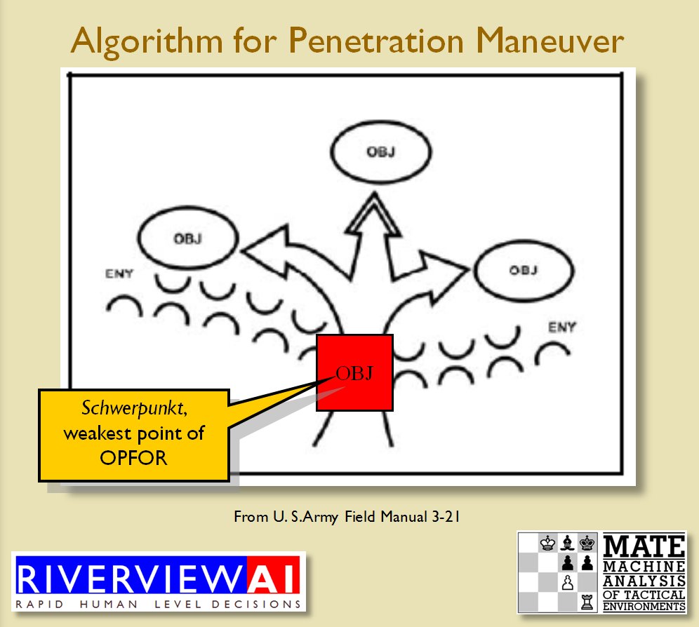
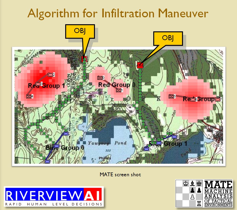
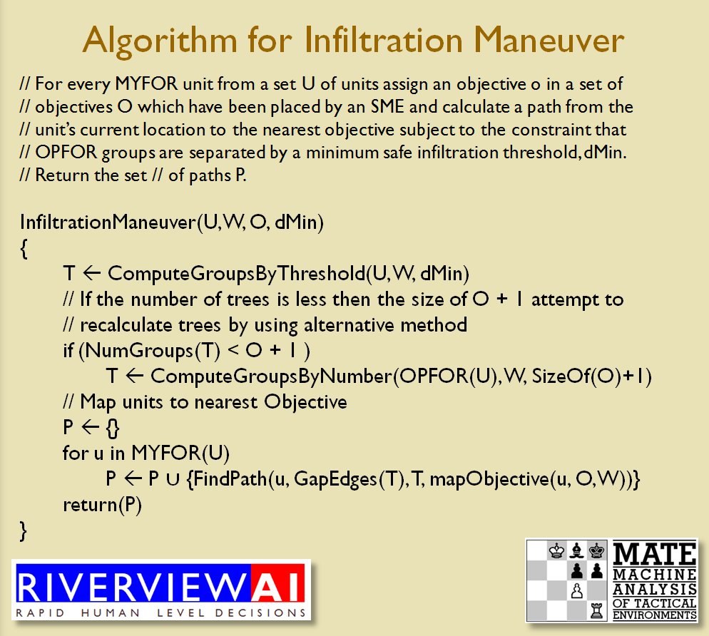
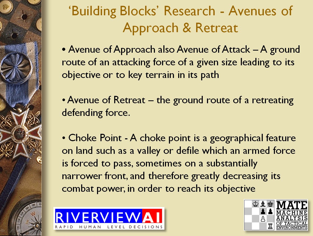
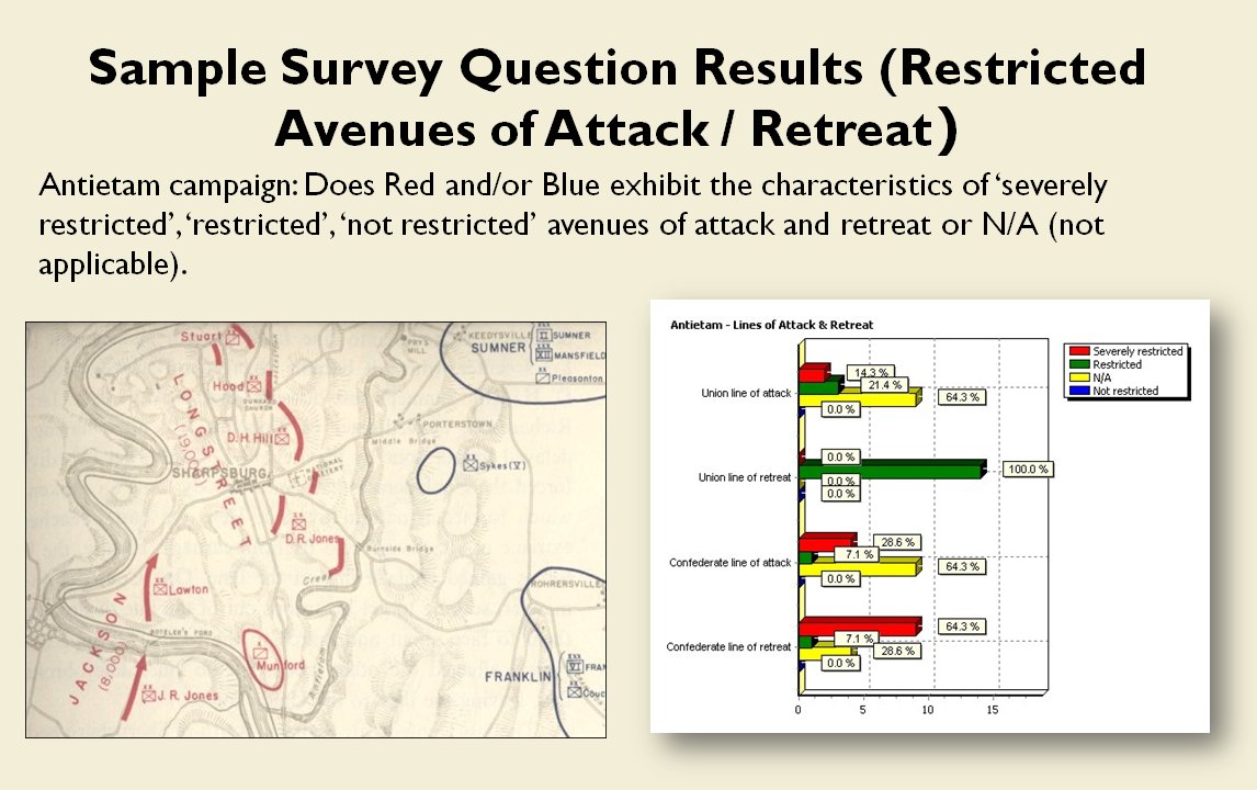
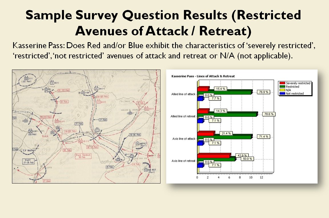
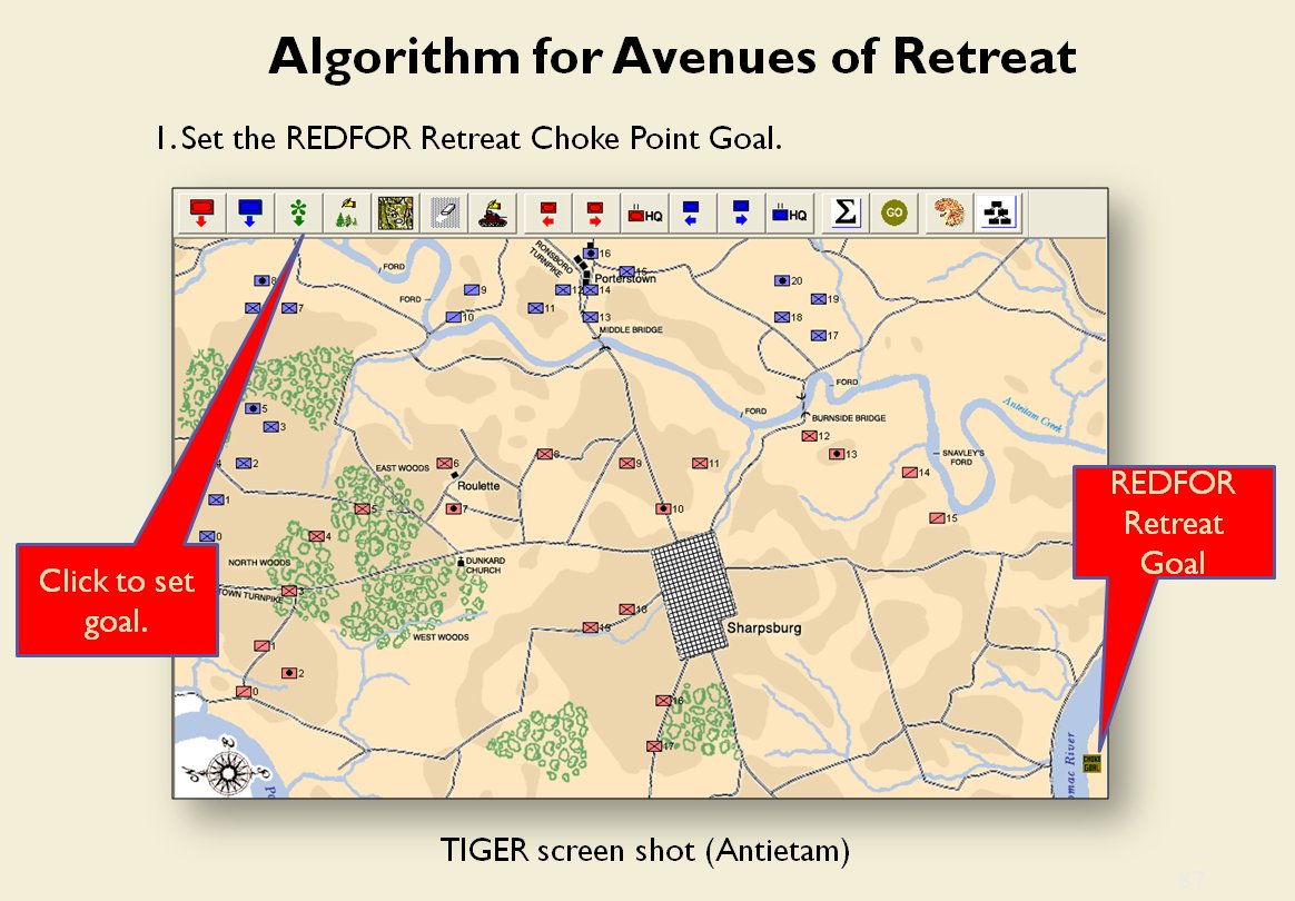
In my previous three posts on computational military reasoning (tactical artificial intelligence) we introduced my algorithms for detecting the absence or presence of anchored and unanchored flanks, interior lines and restricted avenues of attack (approach) and retreat. In this post I present my doctoral research1)TIGER: An Unsupervised Machine Learning Tactical Inference Generator which can be downloaded here which utilizes these algorithms, and others, in the construction of an unsupervised machine learning program that is able to classify the current tactical situation (battlefield) in the context of previously observed battles. In other words, it learns and it remembers.

‘Machine learning’ is the computer science term for learning software (in computer science ‘machine’ often means ‘software’ or ‘program’ ever since the ‘Turning Machine'2)https://en.wikipedia.org/wiki/Turing_machine which was not a physical machine but an abstract thought experiment.

There are two forms of machine learning: supervised and unsupervised machine learning. Supervised machine learning requires a human to ‘teach’ the software. An example of supervised machine learning is the Netflix recommendation system. Every time you watch a show on Netflix you are teaching their software what you like. Well, theoretically. Netflix recommendations are often laughingly terrible (no, I do not want to see the new Bratz kids movie regardless of how many times you keep recommending it to me).

Unsupervised machine learning is a completely different animal. Without human intervention an unsupervised machine learning program tries to make sense of a series of ‘objects’ that are presented to it. For the TIGER / MATE program, these objects are battles and the program classifies them into similar clusters. In other words, every time TIGER / MATE ‘sees’ a new tactical situation it asks itself if this is something similar (and how similar) to what it’s seen before or is it something entirely new?

I use convenient terms like ‘a computer tries to make sense of’ or a ‘computer sees’ or a ‘computer thinks’ but I’m not trying to make the argument that computers are sentient or that they see or think. These are just linguistic crutches that I employ to make it easier to write about these topics.

So, a snapshot of a battle (the terrain, elevation and unit positions at a specific time) is an ‘object’ and this object is described by a number of ‘attributes’. In the case of TIGER / MATE, the attributes that describe a battle object are:

  • Interior Line Value
  • Anchored / Unanchored Flank Value
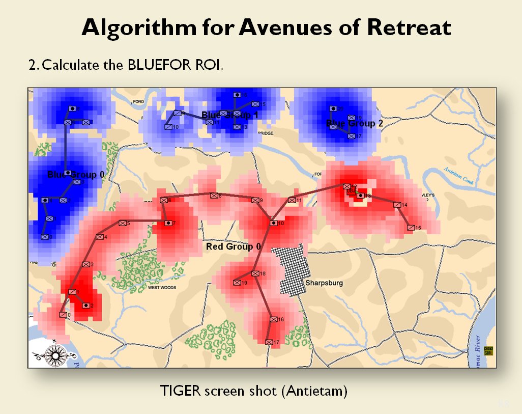
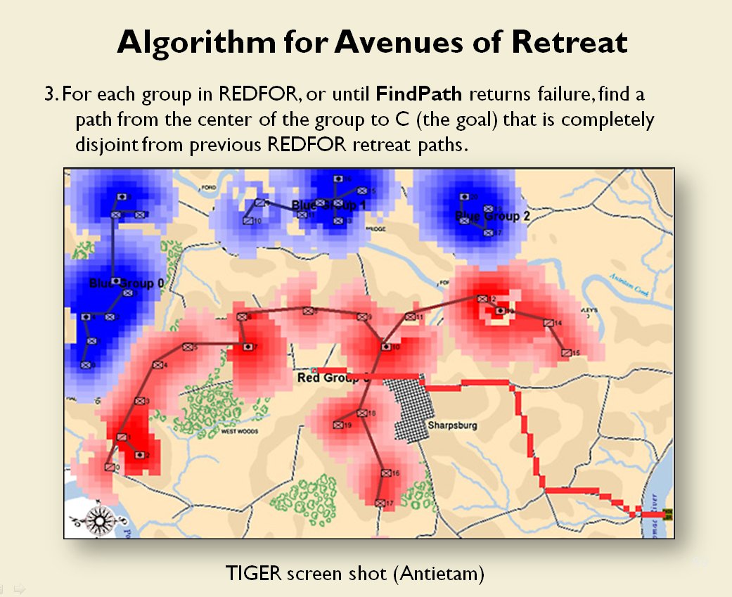
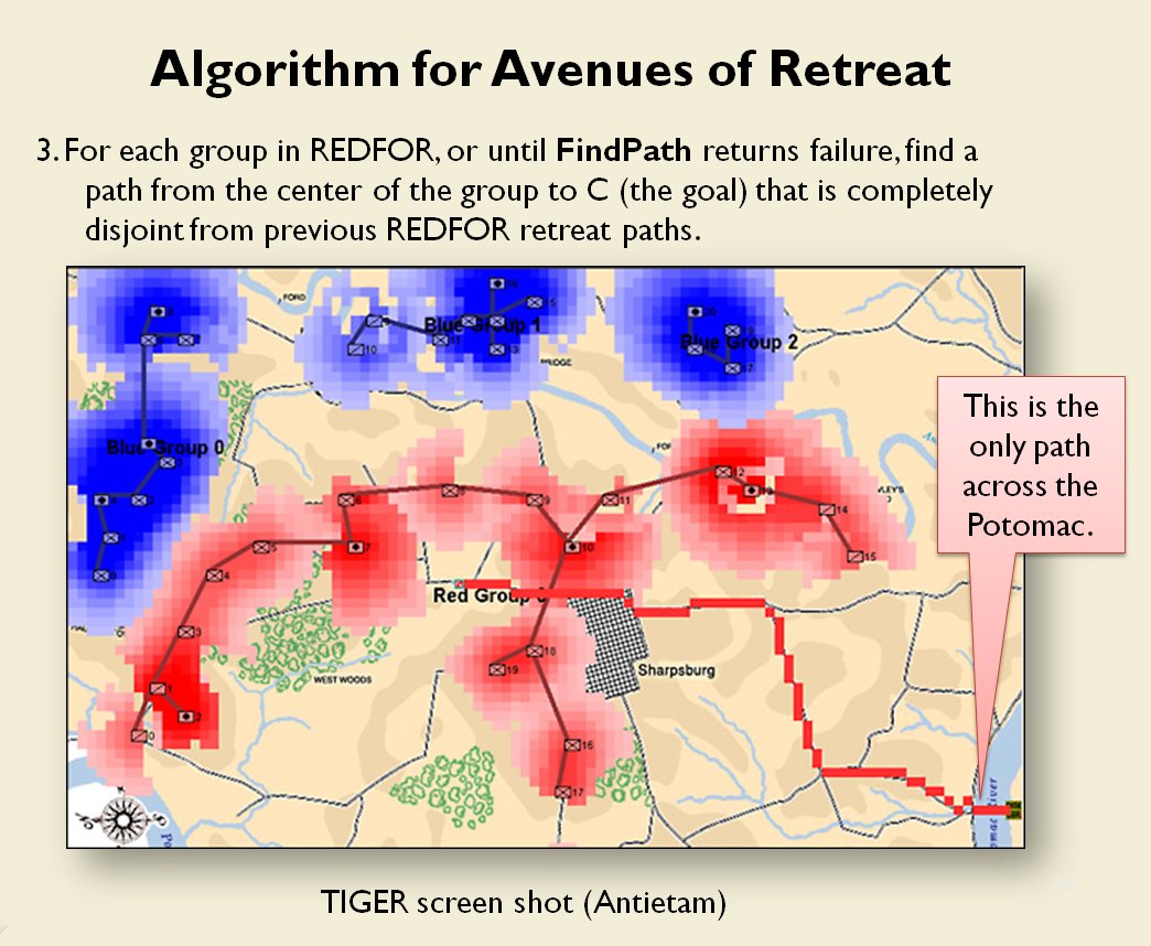
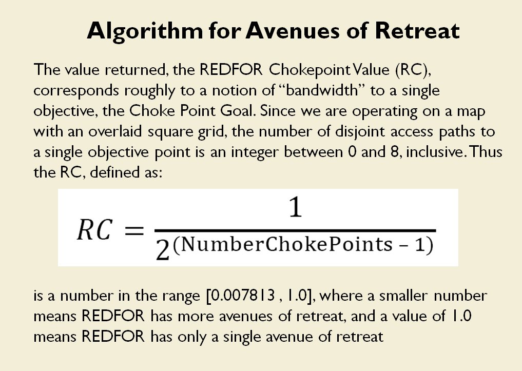
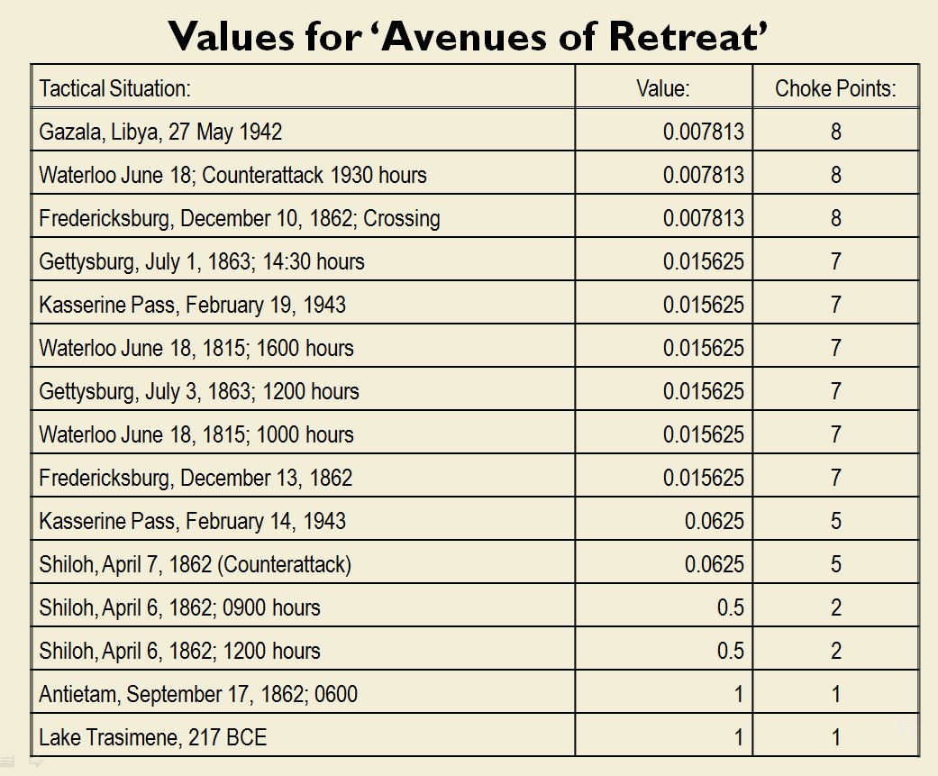
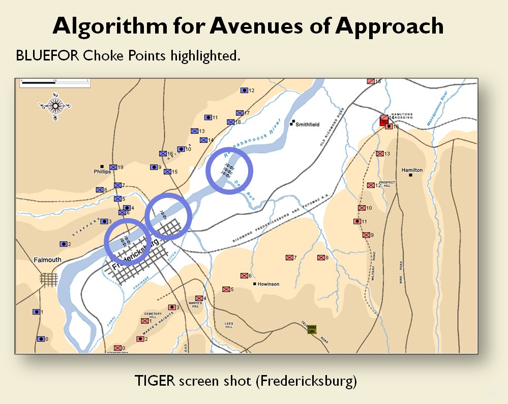
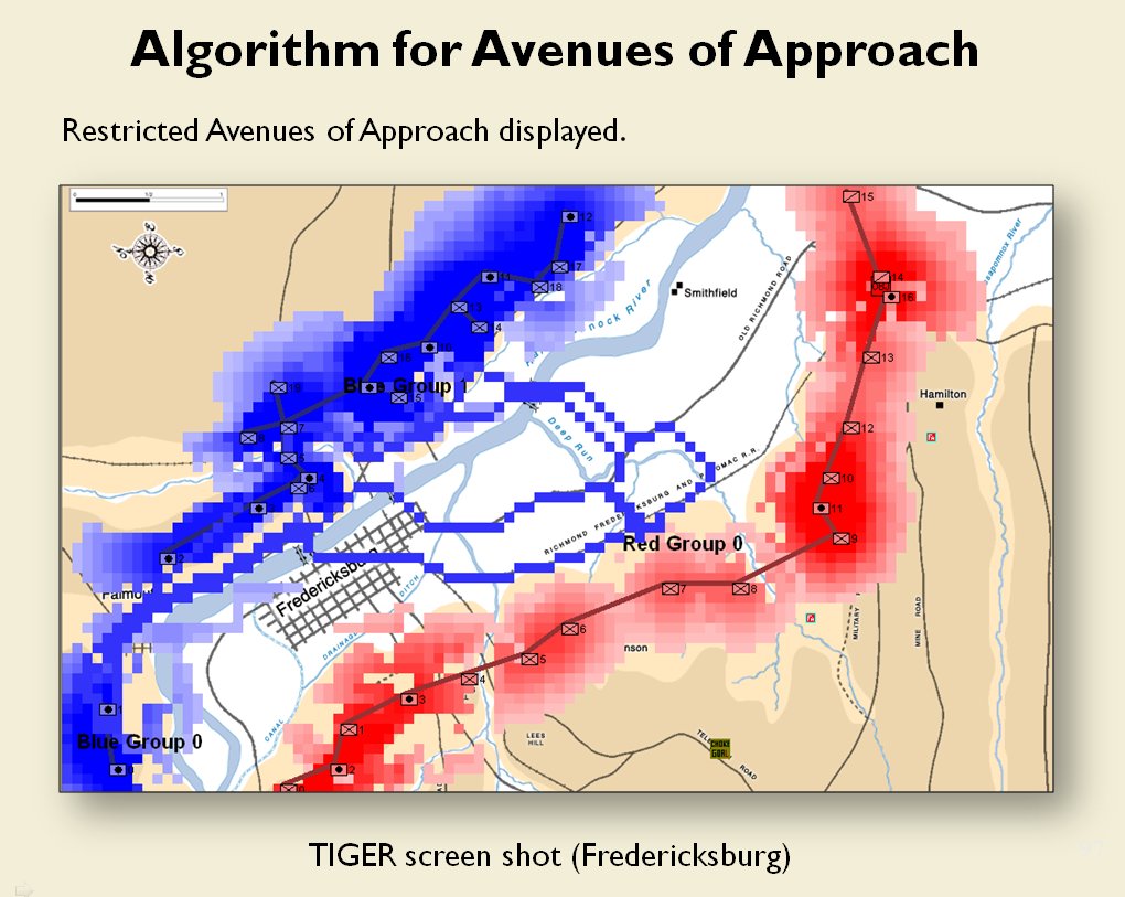
  • REDFOR (Red Forces) Choke Points Value
  • BLUEFOR (Blue Forces) Choke Points Value
  • Weighted Force Ratio
  • Attack Slope

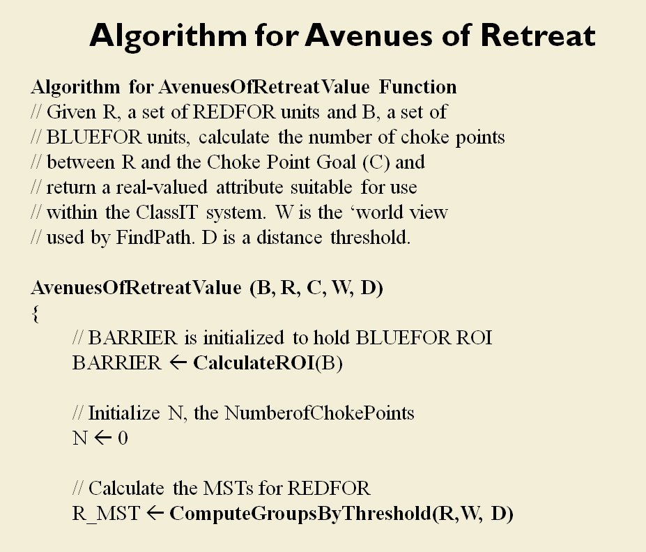
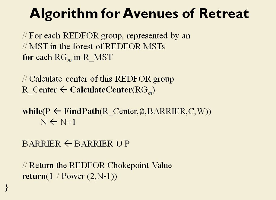
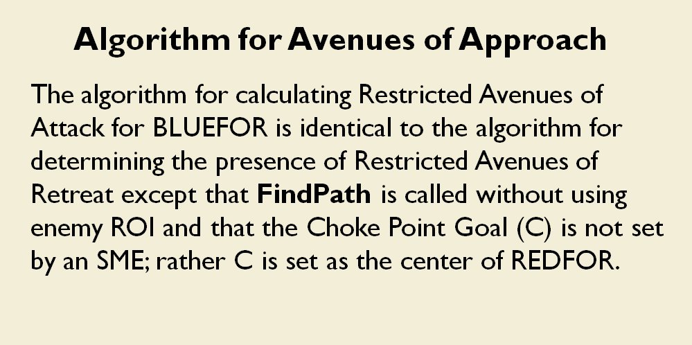
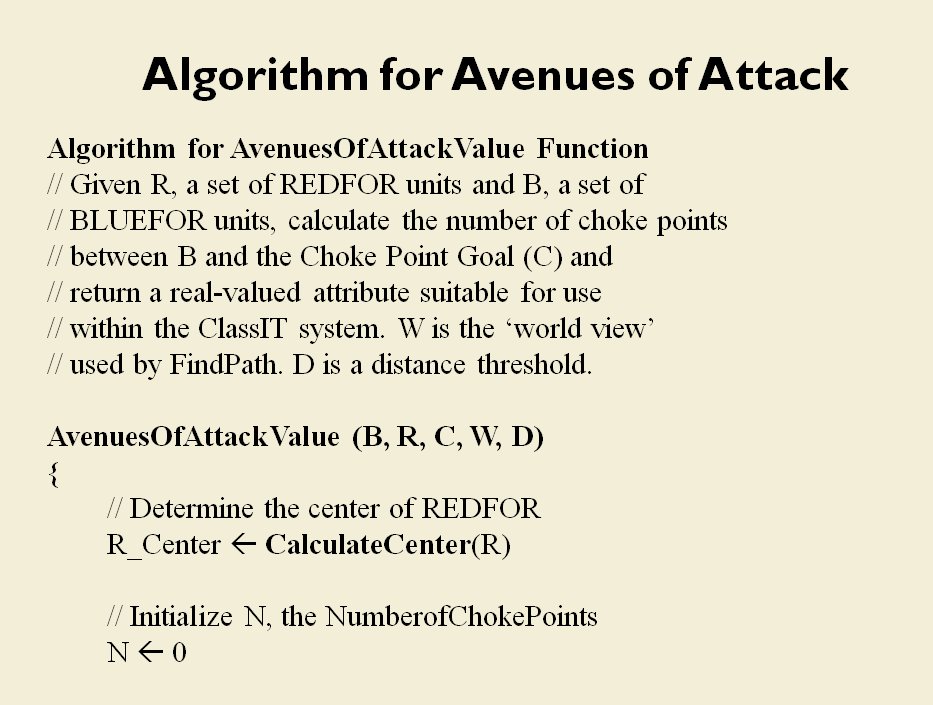
The algorithms for calculating the metrics for the first four attributes were discussed in the three previous blog posts cited above. The algorithms for calculating the Weighted Force Ratio and Attack Slope metrics are straightforward: Weighted Force Ratio is the strength of Red over the strength of Blue weighted by unit type and the Attack Slope is just that: the slope (uphill or downhill) that the attacker is charging over.

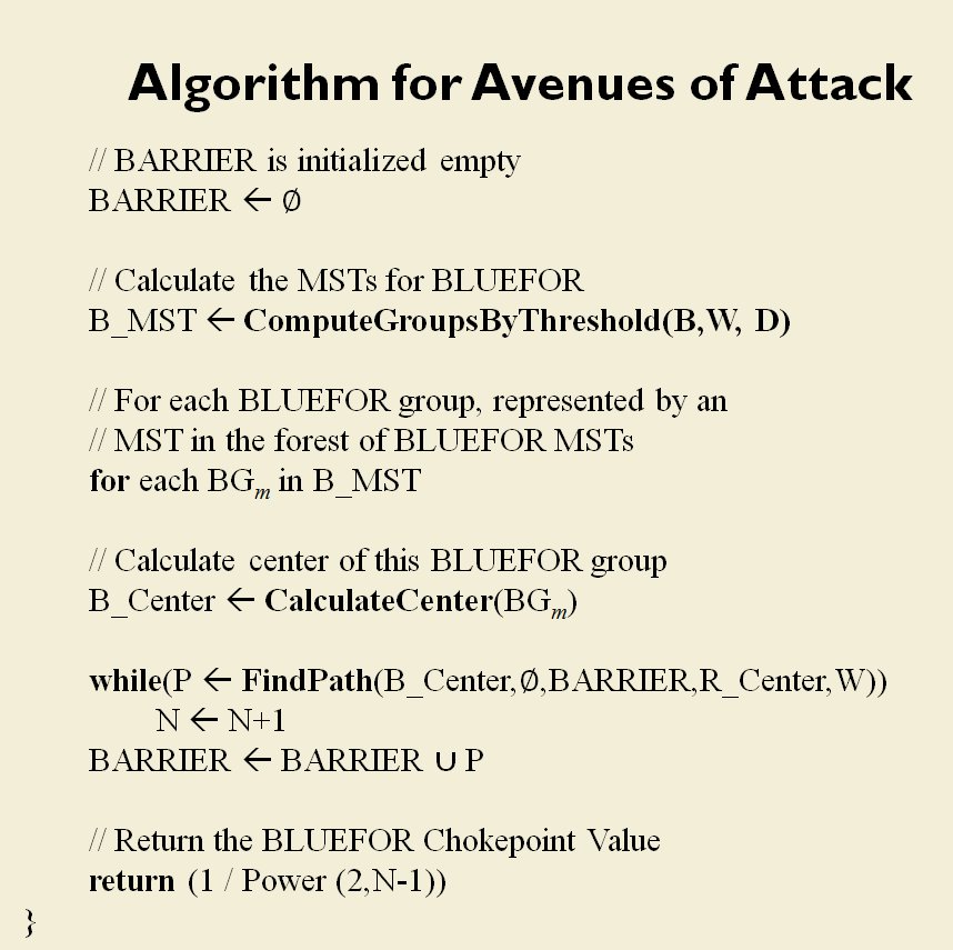
TIGER / MATE constructs a hierarchical tree of battlefield snapshots. This tree represents the relationship and similarity of different battlefield snapshots. For example, two battlefield situations that are very similar will appear in the same node, while two battlefield situations that are very different will appear in disparate nodes. This will be easier to follow with a number of screen shots. Unfortunately, we first have to introduce the Category Utility Function.

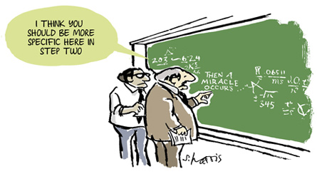
So, first let me apologize for all the math. It isn’t necessary for you to understand how the TIGER / MATE unsupervised machine learning process works, but if I don’t show it I’m guilty of this:

The Category Utility Function (or CU, for short) is the equation that determines how similar or dissimilar too objects (battlefields) are. This it the CU function:

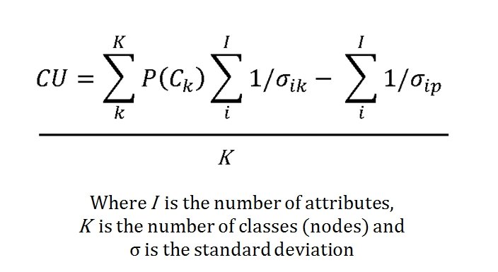
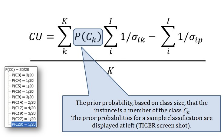
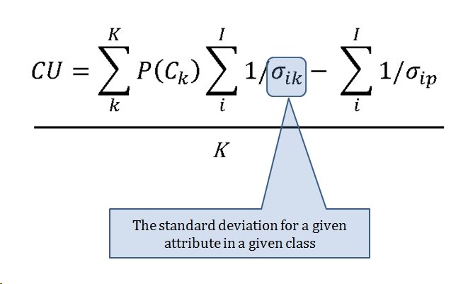
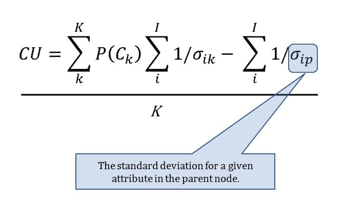
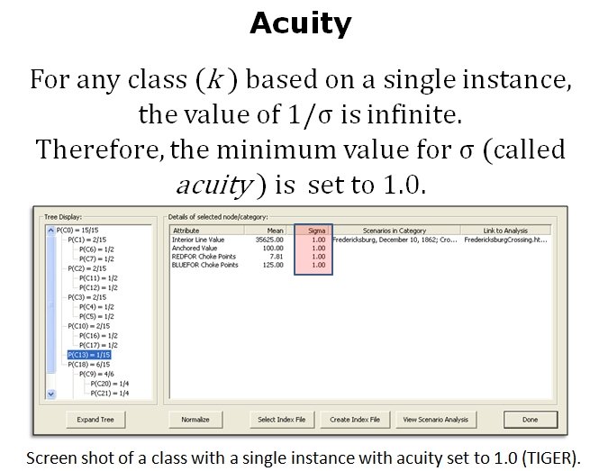
‘Acuity’ is the concept of the minimum value that separates two ‘instances’ (in our case, battles). It has to have a value of 1.0 or very bad things will happen.


So, let’s recap what we’ve got:

  • A series of algorithms that analyze a battlefield and return values representing various conditions that SMEs agree are significant (flanks, attack and retreat routes, unit strengths, etc., etc).
  • A Category Utility Function (CU) that uses the products of these algorithms to determine how similar analyzed battlefields are.

So now, we just need to put this all together. A battlefield (tactical situation) is analyzed by TIGER / MATE. It is ‘fed’ into the unsupervised machine learning function and, using the Category Utility Function one of four things happen:

  1. All the children of the parent node are evaluated using the CU function and the object (tactical situation)is added to an existing node with the best score.
  2. The object is placed in a new node all by itself.
  3. The two top-scoring nodes are combined into a single node and the new object is added to it.
  4. A node is divided into several nodes with the new objected to one of them.

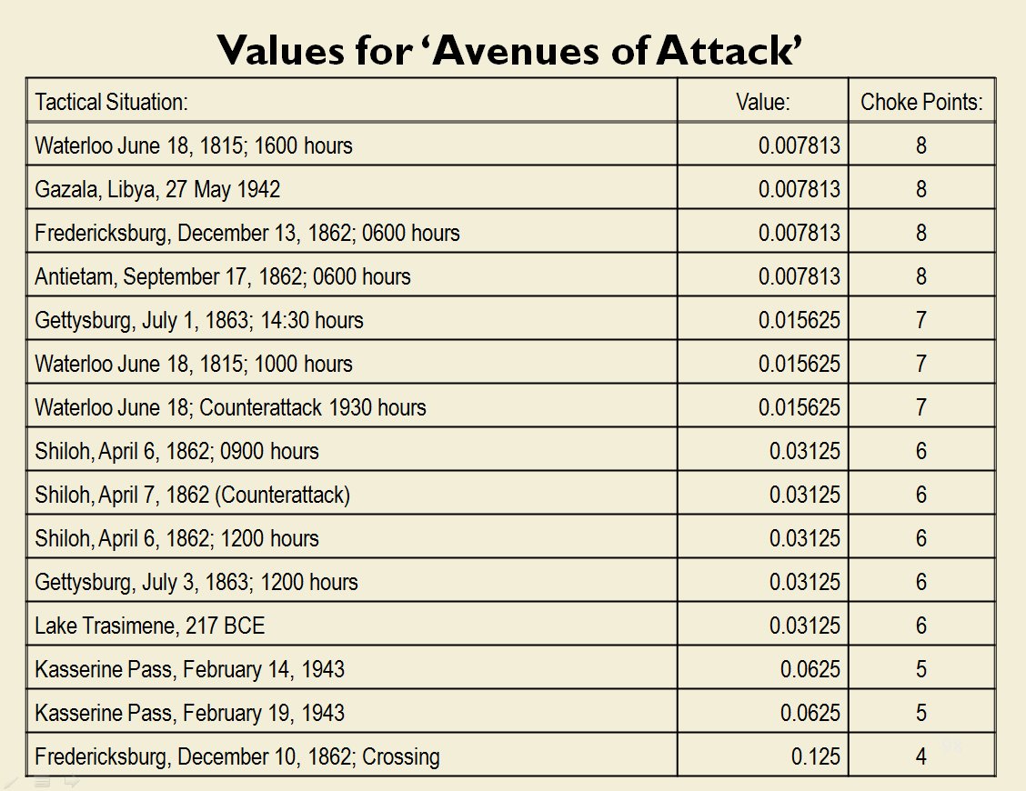
These rules (above) construct a hierarchical tree structure. TIGER was fed 20 historical tactical situations (below):

  1. Kasserine Pass February 14,1943
  2. KasserinePass February 19, 1943
  3. Lake Trasimene, 217 BCE
  4. Shiloh Day 2
  5. Shiloh Day 1, 0900 hours
  6. Shiloh Day 1, 1200 hours
  7. Antietam 0600 hours
  8. Antietam 1630 hours
  9. Fredericksburg, December 10
  10. Fredericksburg, December 13
  11. Chancellorsville May 1
  12. Chancellorsville May 2
  13. Gazala
  14. Gettysburg, Day 1
  15. Gettysburg, Day 2
  16. Gettysburg, Day 3
  17. Sinai, June 5
  18. Waterloo, 1000 hours
  19. Waterloo, 1600 hours
  20. Waterloo, 1930 hours

In addition to these 20 historical tactical situations five hypothetical situations were created labeled A-E. This is the resulting tree which TIGER created:

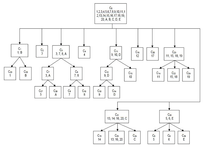
The hierarchical tree created by TIGER from 20 historical and 5 hypothetical tactical situations. The numbers in the nodes refer to the above legend. Battles placed in the same nodes are considered very similar by TIGER. Click to enlarge.

If we look at the tree that TIGER constructed we can see that it placed Shiloh Day 1 0900 hours and Shiloh Day 1 1200 hours together in cluster C35. Indeed, as we look around the tree we observe that TIGER did a remarkable job of analyzing tactical situations and placing like with like. But, that’s easy for me to say, I wrote TIGER. My opinion doesn’t count. So we asked 23 SMEs which included:

  • 7 Professional Wargame Designers
  • 14 Active duty and retired U. S. Army officers including:
  • Colonel (Ret.) USMC infantry 5 combat tours, 3 advisory tours
  • Maj. USA. (SE Core) Project Leader, TCM-Virtual Training
  • Officer at TRADOC (U. S. Army Training and Doctrine Command)
  • West Point; Warfighting Simulation Center
  • Instructor, Dept of Tactics Command & General Staff College
  • PhD student at RMIT
  • Tactics Instructor at Kingston (Canada)

And in a blind survey asked them not what TIGER did but what they would do. For example:

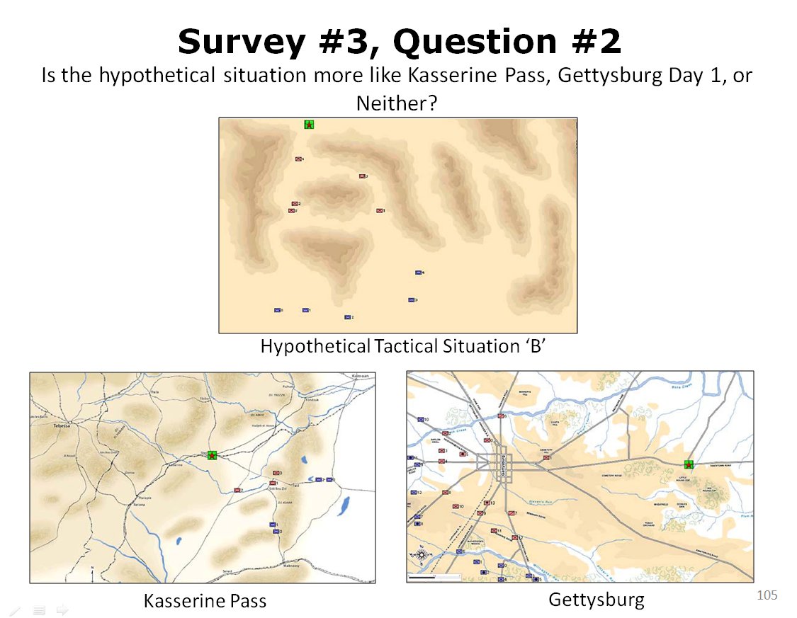
Twenty-three SMEs were asked this question: is this hypothetical tactical situation (top) more like Kasserine Pass or Gettysburg?. Click to enlarge.

And this is how the responded:

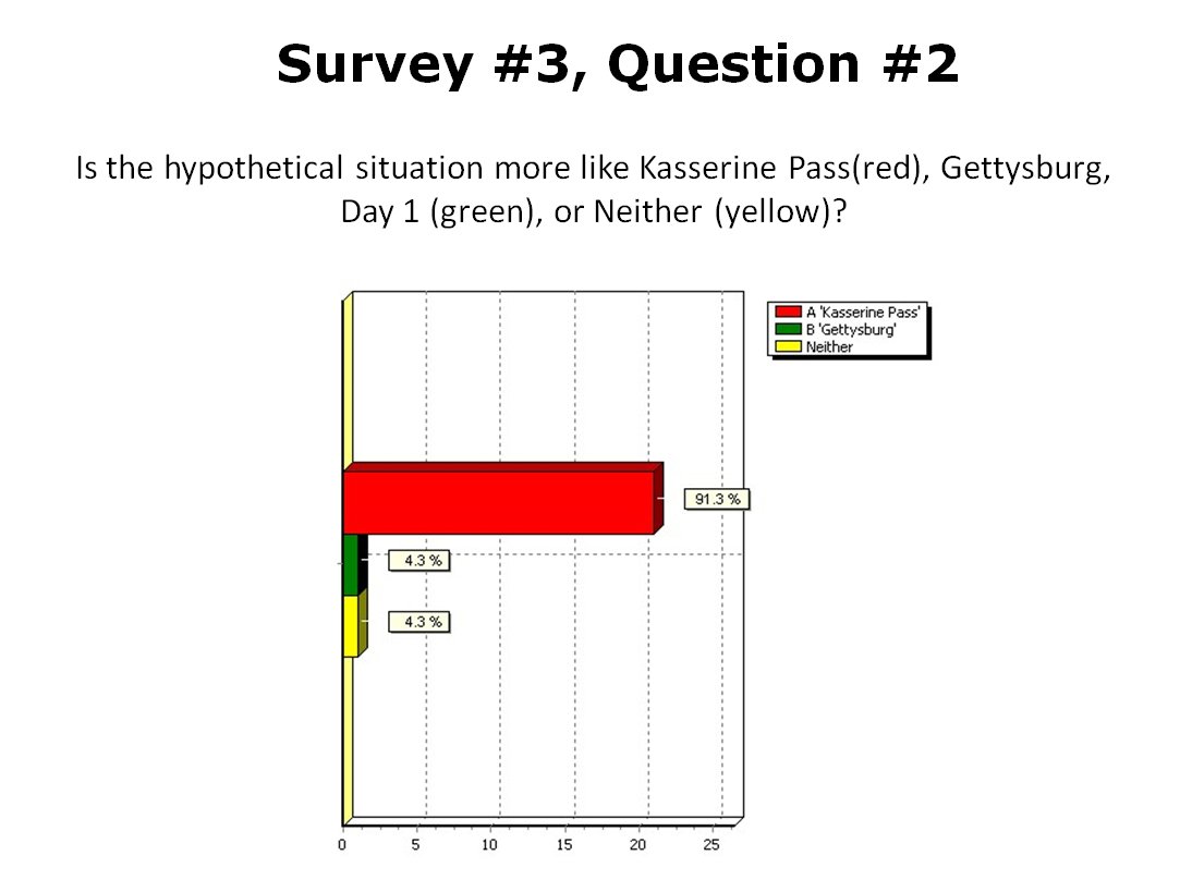
Results from 23 SMEs answering the above question. Overwhelmingly the SMEs agreed that that the hypothetical tactical situation was most like the battle of Kasserine Pass.

So, 91.3% of SMEs agreed that the hypothetical tactical situation was more like Kasserine Pass than Gettysburg Day 1. Unbeknownst to the SMEs TIGER had already classified these three tactical situations like this:

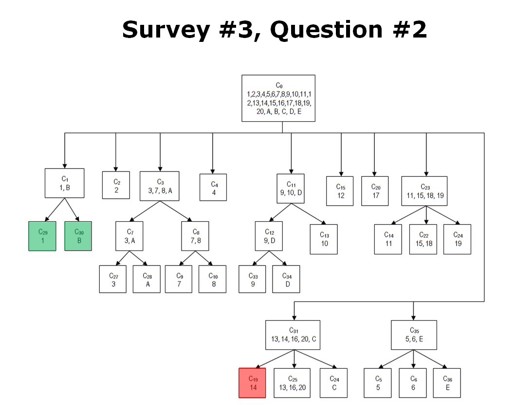
How TIGER classified Kasserine Pass (1), Gettysburg Day 1 (14) and a hypothetical tactical situation (B). The cluster C1 contains two tactical situations that both have restricted avenues of attack caused by armor traveling through narrow mountainous passes. These passes also partially create restricted avenues of retreat. REDFOR does not have anchored flanks.Click to enlarge.

In conclusion: over the last four blog posts about Computational Military Reasoning we have demonstrated:

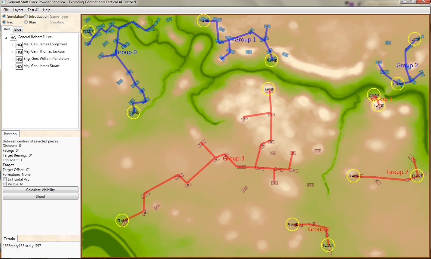
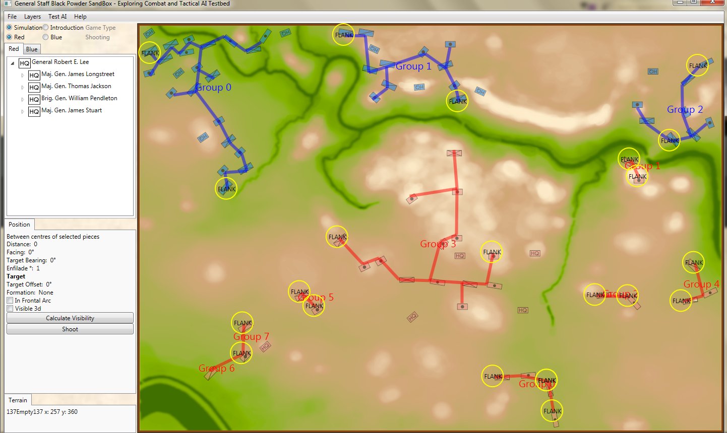
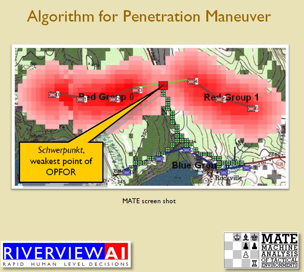
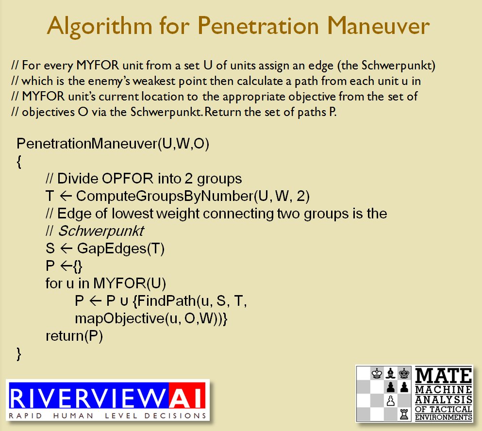
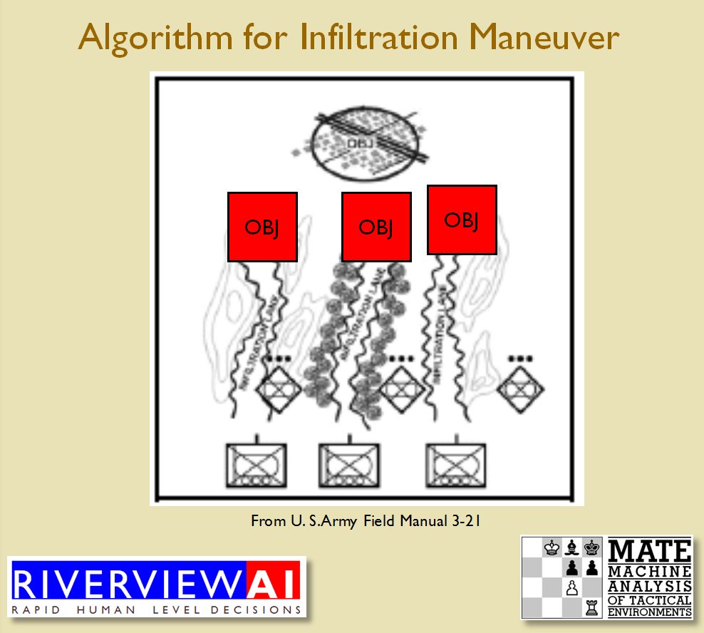
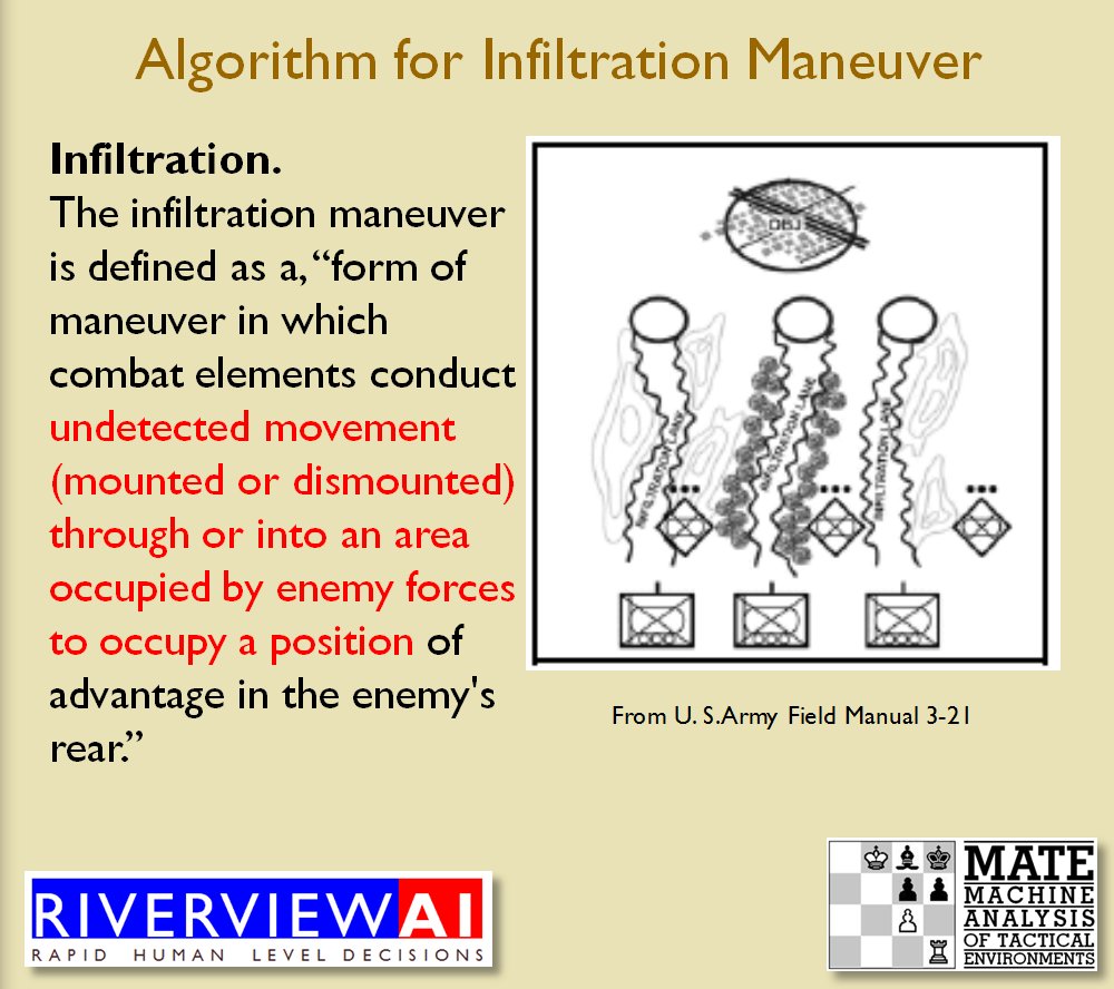
  • Algorithms for analyzing a battlefield (tactical situation).
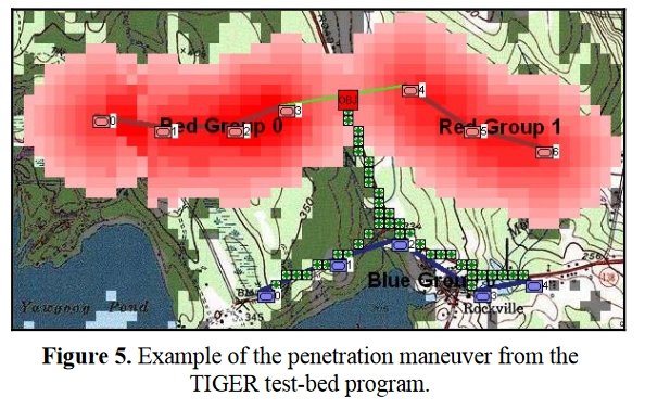
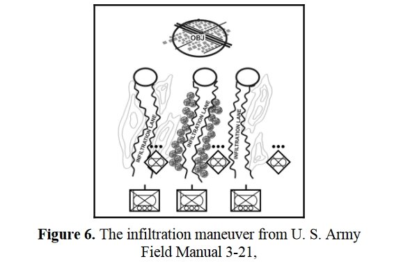
  • Algorithms for implementing offensive maneuvers.
  • An Unsupervised Machine Learning system for classifying tactical situations and clustering like situations together. Furthermore, this system is never-ending and as it encounters new tactical situations it will continue this process which enables the AI to plan maneuvers based on previously observed and annotated situations.

This is the AI that will be used in General Staff. It is unique and revolutionary. No computer military simulation – either commercially available or any military simulation used by any of the world’s armies – employ an AI of this depth.

As always, please feel free to contact me directly with questions or comments. You can use our online email form here or write to me directly at Ezra [at] RiverviewAI.com.

References

References
1 TIGER: An Unsupervised Machine Learning Tactical Inference Generator which can be downloaded here
2 https://en.wikipedia.org/wiki/Turing_machine

Computational Military Reasoning (Tactical Artificial Intelligence) Part 3

In my two previous blog posts on the subject of battlefield analysis (computational military reasoning and tactical artificial intelligence) I discussed how the TIGER1)Tactical Inference Generator / MATE2)Machine Analysis of Tactical Environments program can identify certain key tactical positions such as anchored / unanchored flanks and restricted / unrestricted avenues of approach (attack) and retreat. In this blog post we will look at how TIGER / MATE performs analysis of frontages and implements the infiltration and penetration maneuvers.

MATE / TIGER employs a number of ‘building block’ algorithms that are used in various tactical and battlefield analysis algorithms. One set of building block algorithms are the Grouping algorithms that determine weaknesses in frontages. The following slides are from an unclassified briefing that I gave to DARPA (the Defense Advanced Research Project Agency) on my MATE program (funded by DARPA research grant W911NF-11-200024):

All slides can be enlarged by clicking on them. Note: OPFOR = Opposition Forces. In all of these slides OPFOR are the red units.

With the above building block algorithms we can calculate the optimum part of OPFOR’s frontage to set as the Schwerpunkt. Schwerpunkt is a German word meaning, “the point of maximum effort.” The term was used in blitzkrieg planning to specify, “the center of gravity, point of main effort, where a decisive result was to be achieved.”

Using the above algorithms we can now calculate the Schwerpunkt for implementing the penetration and infiltration maneuvers. The following slides are from an unclassified briefing that I gave to DARPA (the Defense Advanced Research Project Agency) on my MATE program (funded by DARPA research grant W911NF-11-200024): All slides can be enlarged by clicking on them.

The Five Canonical Offensive Maneuvers are from the U. S. Army Field Manual 3-21 which is available online. As always, if you have any questions please feel free to email me.

References

References
1 Tactical Inference Generator
2 Machine Analysis of Tactical Environments

Computational Military Reasoning (Tactical Artificial Intelligence) Part 2

In my last blog post I described how the TIGER / MATE programs classified battles (in computer science terms ‘objects’) based on attributes and that anchored or unanchored flanks was one such attribute. After demonstrating the algorithm for calculating the presence or absence of anchored flanks we saw how the envelopment and turning tactical maneuvers were implemented. In this blog post we will look at another attribute: restricted avenues of attack and restricted avenues of retreat.

The only avenue of retreat from the Battle of First Bull Run back to Washington was over a narrow Stone Bridge. When a wagon overturned panic ensued. Library of Congress.

One classic example of a restricted avenue of retreat was the narrow stone bridge crossing Cub Run Creek which was the only eastern exit from the First Bull Run battlefield. The entire Union army would have to pass over this bridge as it fell back on Washington, D.C. When artillery fire caused a wagon to overturn and block the bridge, panic ensued.

At the battle of Antietam Burnside tried to force his entire corps over a narrow bridge to attack a Confederate position on the hill directly above. The bridge was famously carried by the 51st New York Infantry and 51st Pennsylvania Infantry who demanded restoration of their whiskey rations in return for this daring charge. From the original Edwin Forbes drawing. Click to enlarge.

Burnside’s Bridge at the battle of Antietam is a famous example of a restricted avenue of attack. Burnside was unaware that Snavely Ford was only 1.4 miles south of the stone bridge and allowed a back door into the Confederate position. Consequently, he continued to throw his corps across the bridge with disastrous results.

How to determine if there is a restricted line of attack or a restricted line of retreat on a battlefield

From the perspective of computer science restricted avenues of retreat and restricted avenues of attack are basically the same problem and can be solved with a similar algorithm.

As before we must first establish that there is agreement among Subject Matter Experts (SMEs) of the existence of – and the ability to quantify – the attributes of ‘Avenue of Attack’, ‘Avenue of Retreat’ and ‘Choke Point’.

The following slides are from an unclassified briefing that I gave to DARPA (the Defense Advanced Research Project Agency) on my MATE program (funded by DARPA research grant W911NF-11-200024):

All slides can be enlarged by clicking on them.

Now that we have determined if there is a restricted avenue of attack the next blog post will discuss what to do with this information; specifically the implementation of the infiltration and penetration offensive maneuvers.

As always, if you have any questions please feel free to email me.

References:

TIGER: An Unsupervised Machine Learning Tactical Inference Generator, Sidran, D. E. Download here.

Computational Military Reasoning (Tactical Artificial Intelligence) Part 1

I coined the phrase ‘computational military reasoning’ in grad school to explain what my doctoral thesis in computer science was about. ‘Computational reasoning’ is a formal method for solving problems (technically, you don’t even need a computer). But, for our purposes it means a computer solving ‘human-level’ problems. A classic example of this would be calculating the fastest route on a map between two points. In computer science we call this a ‘least weighted path’ algorithm and I did my Q (Qualifying) Exam on this subject. I have also written extensively on the subject including these blog posts.

So, ‘computational military reasoning’ is a, “computer solving human-level military problems.” Furthermore, we can divide computational military reasoning into two subcategories: strategic and tactical (Russian military dogma also adds a third category, ‘grand strategy’); however, for now, let’s concentrate on tactical artificial intelligence; or battlefield decisions.

Tactical AI is divided into two parts: analyzing – or reading – the battlefield and acting on that information by creating a set coherent orders (commonly known as a COA or Course of Action) that exploit the weaknesses in our enemy’s position that we have found during our battlefield analysis.


It is said that as Napoleon traveled across Europe with his staff he would question them about the terrain that they were passing; “Where is the best defensive position? What are the best attack routes?” Where would you position artillery? What ground is favorable for cavalry attack?”

We take it for granted that such analysis of terrain and opposing forces positioned upon it is a skill that can be taught to humans. My doctoral research 1)TIGER: An Unsupervised Machine Learning Tactical Inference Generator; This thesis can be downloaded free of charge here. successfully demonstrated the hypothesis that an unsupervised machine learning program could also learn this skill and perform battlefield analysis that was statistically indistinguishable2)Using a one sided Wald test resulted in  p = 0.0001.In other words, it was extremely unlikely that TIGER was ‘guessing correctly’. from analyses performed by Subject Matter Experts (SMEs) such as instructors at West Point and active duty combat command officers.

Supervised & Unsupervised Machine Learning

Netflix recommendations are a supervised learning program. Every time you ‘like’ a movie the program ‘learns’ that you like ‘documentaries’; for example. Any program that has you ‘like’ or ‘dislike’ offerings is a supervised learning program. You are the supervisor and by clicking on ‘like’ or ‘dislike’ you are teaching the program.

TIGER is an unsupervised machine learning program. That means it has to figure everything out for itself. Rather than being taught, TIGER is ‘fed’ a series of ‘objects’ that have ‘attributes’ and it sorts them into like categories. For TIGER the objects are snapshots of battlefields.

Screen capture from TIGER. An ‘object’ has been loaded into TIGER for analysis; in this case a ‘snapshot’ of the battle of Antietam at 1630 hours on September 17, 1863. Click to enlarge.

How TIGER perceives the battlefield

When you and I look at a battlefield our brains, somehow, make sense of all the NATO 2525B icons scattered around the topographical map. I don’t know how our brains do it, but this is how TIGER does it:

Screen capture from TIGER: How TIGER converts unit positions into lines and frontages using a Minimum Spanning Tree (MST). Click to enlarge.

By combining 3D Line of Sight with Range of Influence (how far weapons can fire and how accurate they are at greater distances displayed, above, with lighter colors) with a Minimum Spanning Tree algorithm3)Kruskal’s algorithm, https://en.wikipedia.org/wiki/Kruskal%27s_algorithm the above image is how TIGER ‘sees’ the battlefield of Antietam. This is an important first step for evaluating object attributes.

How to determine the attribute of anchored or unanchored flanks

Battlefields are ‘objects’ that are made up of ‘attributes’. One of these attributes is the concept of anchored and unanchored flanks. While anyone who plays wargames probably has a good idea what is meant by a ‘flank’, following formal scientific methods I had to first prove that there was agreement among Subject Matter Experts (SMEs) on the subject. This is from one of the double-blind surveys given to SMEs:

Screen shot from online double-blind survey of Subject Matter Experts on identifying the presence of Anchored and Unanchored Flanks. Click to enlarge.

And their responses to the situation at Antietam:

Subject Matter Experts response to the question of the presence of Anchored or Unanchored flanks at Antietam. Click to enlarge.

And another double-blind survey question asked of the SMEs about anchored or unanchored flanks at Chancellorsville:

Response to double-blind survey question asked of SMEs about anchored and unanchored flanks at Chancellorsville. Click to enlarge.

So, we have now proven that there is agreement among Subject Matter Experts about the concept of ‘anchored’ and ‘unanchored’ flanks and, furthermore, some battlefields exhibit this attribute and others don’t.

Following is a series of slides from a debriefing presentation that I gave to DARPA (Defense Advanced Research Projects Agency) as part of my DARPA funded research grant (W911NF-11-200024) describing the algorithm that MATE (the successor to TIGER) uses to calculate if a flank is anchored or unanchored and how to tactically exploit this situation with a flanking maneuver. This briefing is not classified. Click to enlarge slides.

How to generate a Course of Action for a flank attack

Once TIGER / MATE has detected an ‘open’ or unanchored flank it will then plot a Course of Action (COA) to maneuver its forces to perform either a Turning Maneuver or an Envelopment Maneuver. Returning to the previous DARPA debriefing presentation (Click to enlarge):

MATE analysis of the battle of Marjah (Operation Moshtarak February 13, 2010)

The following two screen captures are part of MATE’s analysis of the battle of Marjah suggesting an alternative COA  (envelopment maneuver) to the direct frontal assault that the U. S. Marine force actually performed at Marjah. Click to enlarge:

Conclusions & Comments about Computational Military Reasoning (Tactical Artificial Intelligence) & Battlefield Analysis (Part 1)

Usually, at this point when I give this lecture, I look out to my audience and ask for questions. I really don’t want to lose anybody and we’ve got a lot more Tactical AI to talk about. So far, I’ve only covered how my programs (TIGER / MATE) analyze a battlefield in one particular way (does my enemy – OPFOR in military terms – have an exposed flank that I can pounce on?) and there is a lot more battlefield analysis to be performed.

It’s easy, as a computer scientist, to use computer science terminology and shorthand for explaining algorithms. But, I worry that the non computer scientists in the audience will not quite get what I’m saying.

Do you have any questions about this? If so, I would really like to hear from you. I’ve been working on this research for my entire professional career (see A Wargame 55 Years in the Making) and, frankly, I really like talking about it. As a TA said to me many years ago when I was an undergrad, “There are no stupid questions in computer science.” So, please feel free to write to me either using our built in form or by emailing me at Ezra [at] RiverviewAI.com

References

References
1 TIGER: An Unsupervised Machine Learning Tactical Inference Generator; This thesis can be downloaded free of charge here.
2 Using a one sided Wald test resulted in  p = 0.0001.In other words, it was extremely unlikely that TIGER was ‘guessing correctly’.
3 Kruskal’s algorithm, https://en.wikipedia.org/wiki/Kruskal%27s_algorithm