
This is what a brilliant game publisher looks like: Marten Davies. I was looking for a photo of Marten from the ’80s and I found this 2019 photo (credit: University of Texas). This is exactly what he looked like in ’87. He hasn’t aged a day.
Marten Davies, my first publisher and still a close friend, was painfully accurate when he said, “Take any time estimate that Ezra gives you and multiply it by three.” Now, in my defense, Marten probably said that because I had a contractual obligation to deliver UMS: The Universal Military Simulator in some insanely short period of time like six months and I actually delivered it in eighteen. To my credit I delivered a #1 game (Europe and US). To Marten’s credit, he was very easy to work with and it remains the best experience of my career. The bottom line was that Marten knew that I needed more time to make a better game and he made sure I got it.
So, what’s the hold-up? Well, that would be me, again.
Specifically, it’s the AI. As many of you know, I’ve been working on AI for wargames for a long time and I was hoping to turn General Staff into a showcase for my work. Some of this has been accomplished 1) Antietam & AI . These are the algorithms that I’ve written about in my doctoral thesis and in various published papers.
The MATE2)Machine Analysis of Tactical Environments, see http://riverviewai.com/ set of tactical AI routines built upwards from low level routines; like 3D Line of Sight (3DLOS) 3) https://www.general-staff.com/tag/3d-line-of-sight/ , Range of Influence (ROI), and least weighted path algorithms 4) https://www.general-staff.com/tag/least-weighted-path-algorithm/ to battlefield analysis 5) Algorithms for Generating Attribute Values for the Classification of Tactical Situations.: http://riverviewai.com/papers/Algorithms-Tactical_Class.pdf , to selection of objectives 6) https://www.general-staff.com/antietam-ai/ , and the implementation of offensive maneuvers 7) Implementing the Five Canonical Offensive Maneuvers in a CGF Environment.:http://riverviewai.com/papers/ImplementingManeuvers.pdf to achieve those objectives.
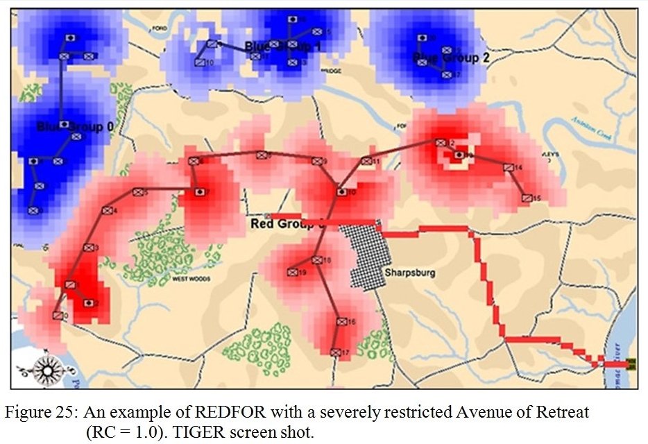
So, given a list of objectives the AI can implement a tactical plan (Course of Action, or COA); but the AI doesn’t have any comprehension of the greater strategic picture. For example, MATE’s analysis of Gettysburg is that Blue8)MATE always labels the attacker as blue (Confederates) should not attack because Red (Union) has interior lines, a superior defensive position, and greater troop strength.
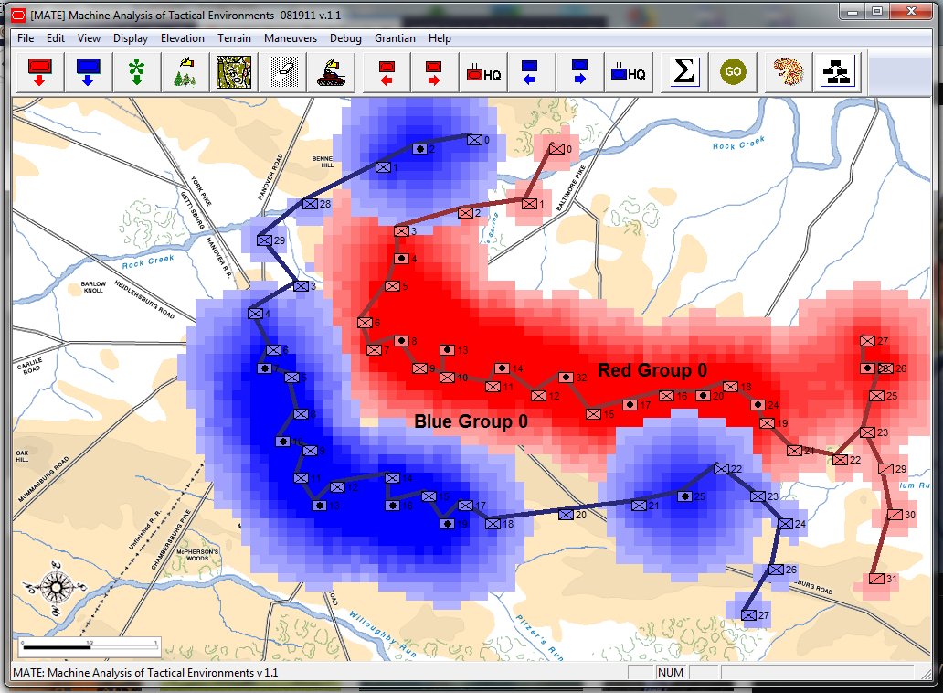
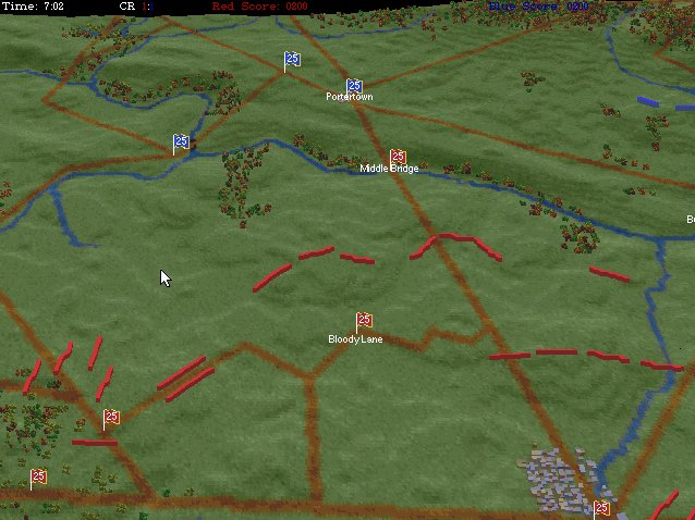
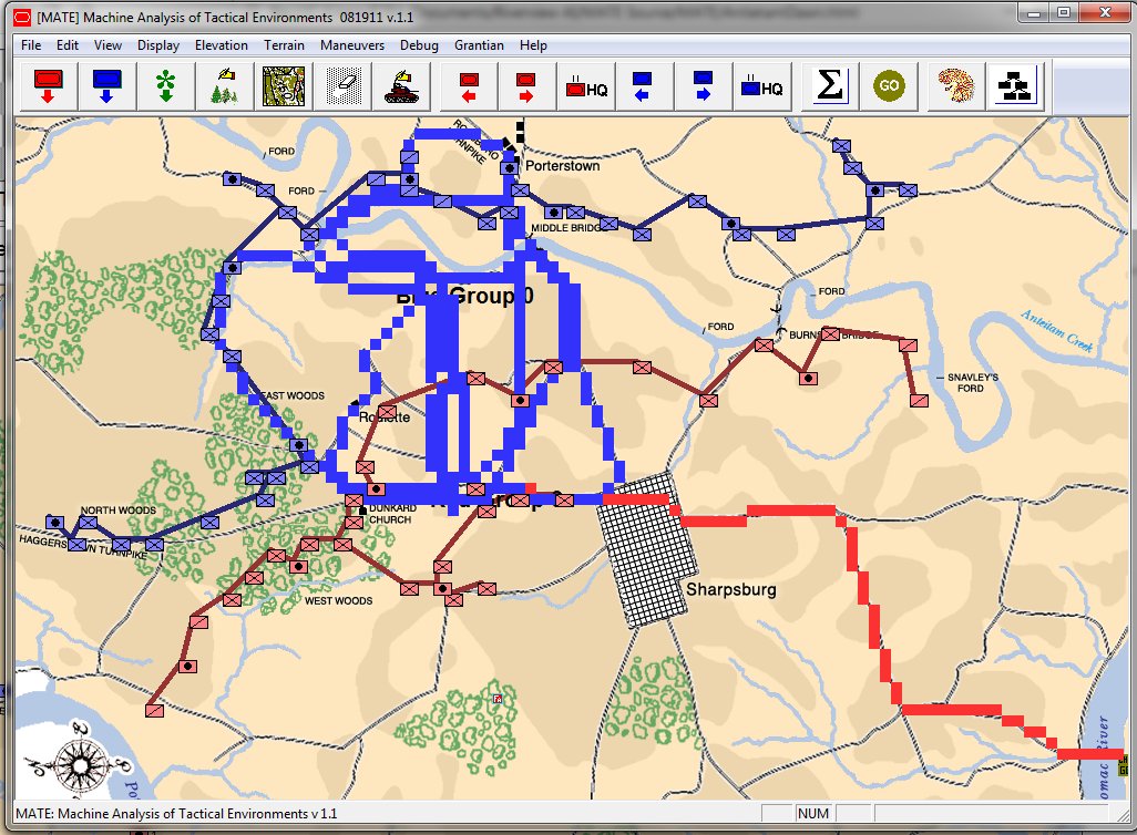
MATE representation of Gettysburg: Confederates (blue), Union (red). MATE screen shot. Click to enlarge,
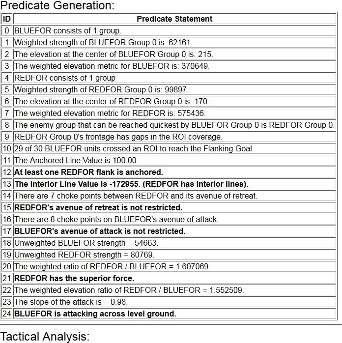
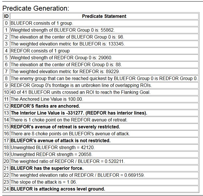
MATE output analysis of Gettysburg. Confederates (BLUEFOR) should not attack because REDFOR (Union) has interior lines, a superior defensive position, and greater troop strength.
But, what the AI doesn’t understand is that the Confederates were desperate for a victory on Union soil which required them to attack at Gettysburg.
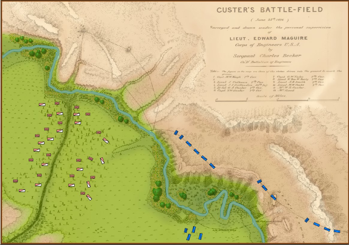
Screen capture of the Battle of Little Bighorn in the General Staff Scenario Editor. Click to enlarge.
Or consider the tactical positions at the battle of the Little Bighorn (above). My goal is to write a human-level tactical AI and, clearly, the historical attack (splitting forces) by Blue (7th Cavalry) against the far superior Red (Native American) forces was very ill advised (perhaps calling into question the definition of ‘human-level tactical AI’).
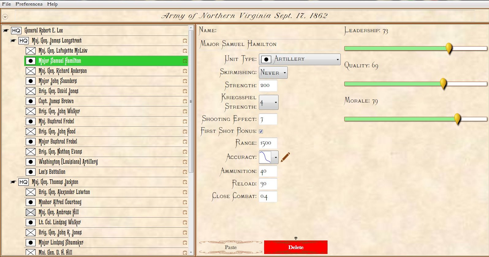
After a lot of thought I realized that I needed to create an AI Editor program. You use the Army Editor to create armies for the General Staff Wargaming System, the Map Editor to create maps, the Scenario Editor to place armies on the map and now you use the AI Editor to quickly and easily select strategies for an army. For example:
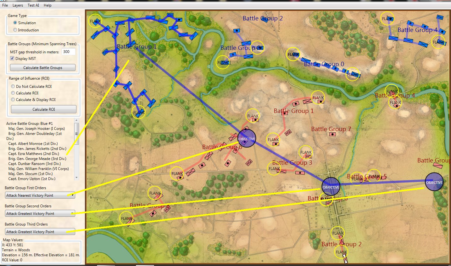
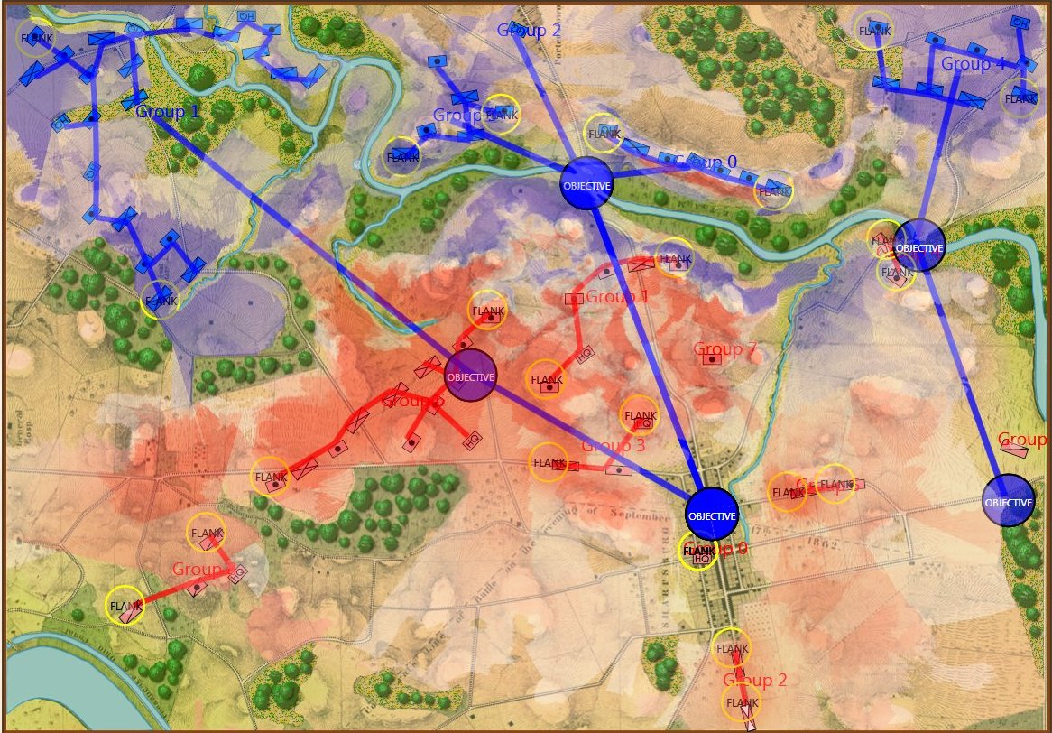
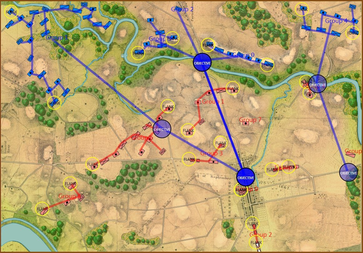
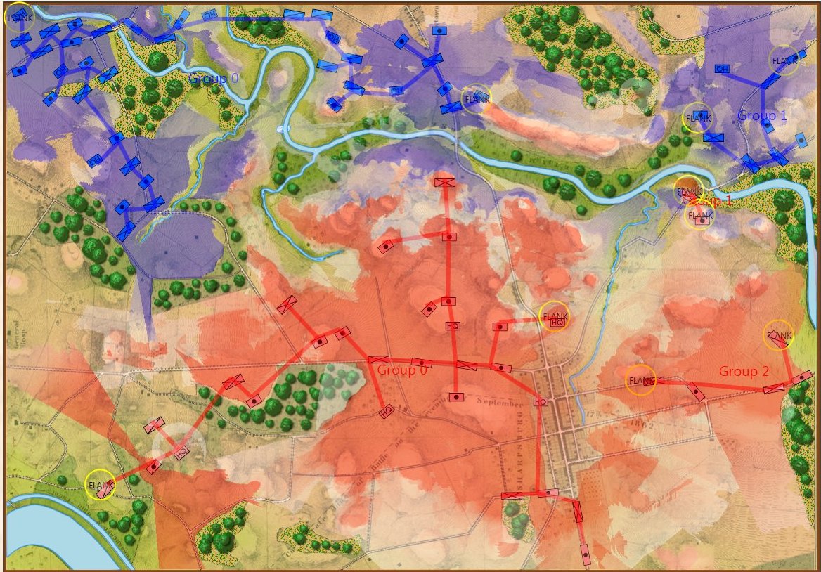
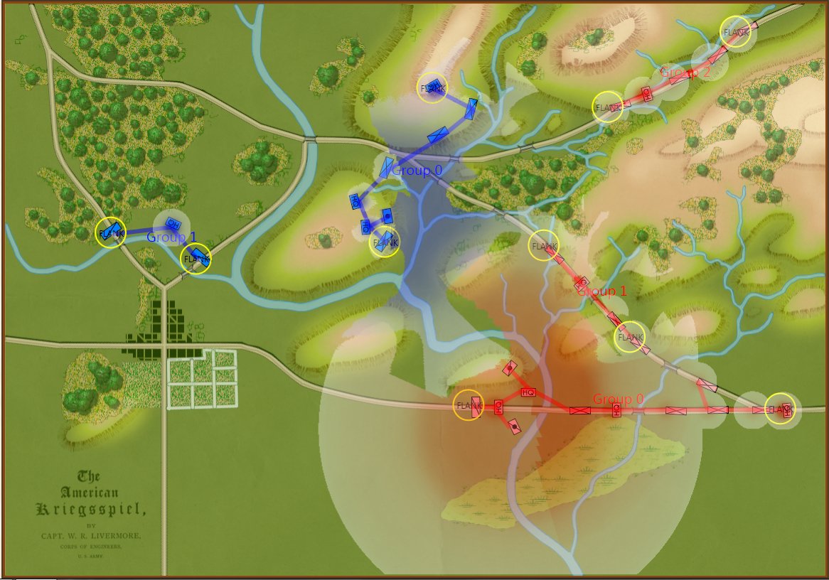
Screen shot of the General Staff AI Editor being used to program AI strategies for the Union forces at Antietam. Click on a battle group and select strategies from the drop down menus. Click to enlarge.
The AI Editor is very easy to use. You just load a scenario (created in the Scenario Editor, of course) tell the AI to separate the units on the field into battle groups (this creates unique groups based on proximity rather than the Order of Battle hierarchy) and then select strategies from the drop down menus. It’s important to note that these units won’t follow the direct paths between objectives; those are just there to show the order of Objectives. The MATE AI algorithms will be engaged to actually move units on the battlefield and implement tactical maneuvers like envelopment and turning attacks. Also, note the AI Editor creates one set of strategies that the AI will follow, if so instructed, when you actually play a simulation. You will also have the option to let the Machine Learning algorithms select strategies as well though these may not follow historical strategies.
It took less than a minute to set up Custer’s strategy at Little Bighorn:
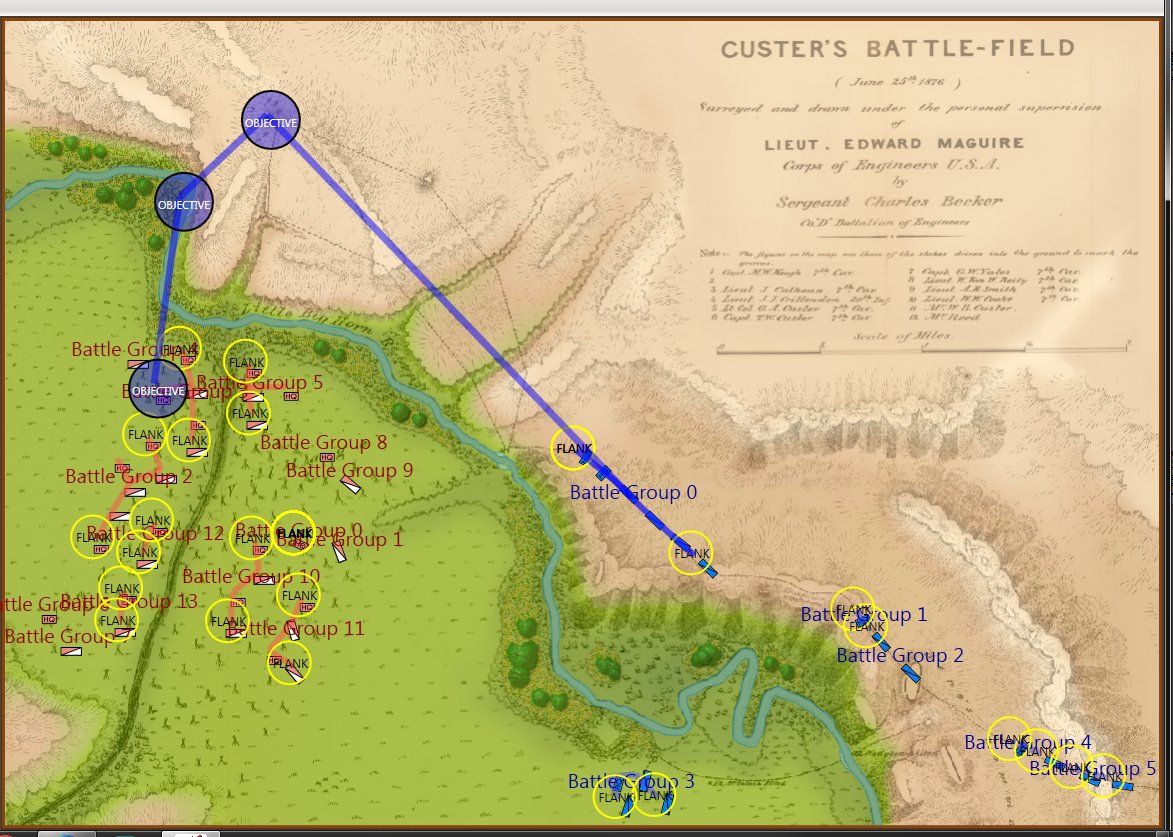
Screen shot from the General Staff AI Editor showing Custer’s historical strategy at Little Bighorn. Click to enlarge.
With the creation of the AI Editor the last piece is in place for the General Staff Wargaming System. We now have nine battlefield maps with more on the way (we’re hoping to ship the finished game with about 20 battlefield maps) and fifteen armies (we hope to have about sixty when we’re finished). We’re now registered with Steam and are getting our ‘store’ set up. We will be using Steam for player vs. player games. With a bit of luck we’re hoping to start player vs. player testing in about sixty days.
As always, please feel free to contact me directly with questions, comments or complaints. I’m sorry for the delay, but we’re creating something that hasn’t been done before and that always takes a bit longer.
References
| ↑1 | Antietam & AI |
|---|---|
| ↑2 | Machine Analysis of Tactical Environments, see http://riverviewai.com/ |
| ↑3 | https://www.general-staff.com/tag/3d-line-of-sight/ |
| ↑4 | https://www.general-staff.com/tag/least-weighted-path-algorithm/ |
| ↑5 | Algorithms for Generating Attribute Values for the Classification of Tactical Situations.: http://riverviewai.com/papers/Algorithms-Tactical_Class.pdf |
| ↑6 | https://www.general-staff.com/antietam-ai/ |
| ↑7 | Implementing the Five Canonical Offensive Maneuvers in a CGF Environment.:http://riverviewai.com/papers/ImplementingManeuvers.pdf |
| ↑8 | MATE always labels the attacker as blue |