Category Archives: Fog of War

Fog of War

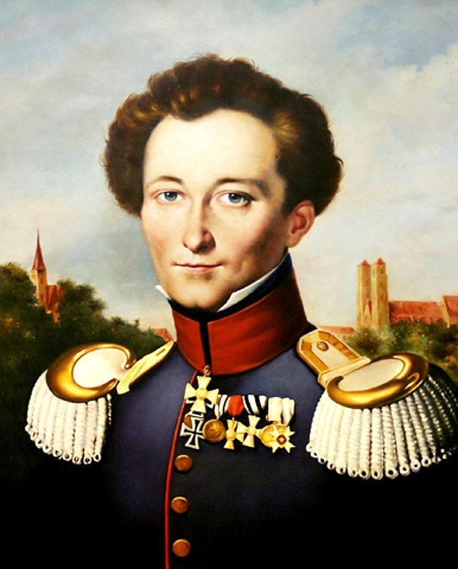
Carl von Clausewitz painted by Karl Wilhelm Wach. Credit Wikipedia. Click to enlarge.

Carl von Clausewitz in his On War wrote, “War is the realm of uncertainty; three quarters of the factors on which action in war is based are wrapped in a fog of greater or lesser uncertainty. A sensitive and discriminating judgment is called for; a skilled intelligence to scent out the truth.” Though Clausewitz never specifically wrote the phrase ‘Fog of War’, the above quote is the source of the term which we abbreviate today as FoW. FoW in the 18th and 19th centuries (the era specifically covered by General Staff: Black Powder) was especially problematic because of the lack of modern day battlefield information gathering techniques such as drones, aircraft and satellites (yes, hot air balloons were used in the Civil War but their actual value during combat was minimal).

General Staff is a wargame that can simulate the FoW experienced by an 18th or 19th century commander and his staff. We use the qualifier ‘can simulate’ because General Staff can run in five different ‘modes’:

Game mode / No Fog of War
Game mode / Partial Fog of War
Simulation mode / No Fog of War
Simulation mode / Partial Fog of War
Simulation mode / Complete Fog of War

Game mode came from a strong desire to create an introductory wargame, with simplified rules, played on historical accurate battlefield maps that could be used to introduce novices to wargaming.

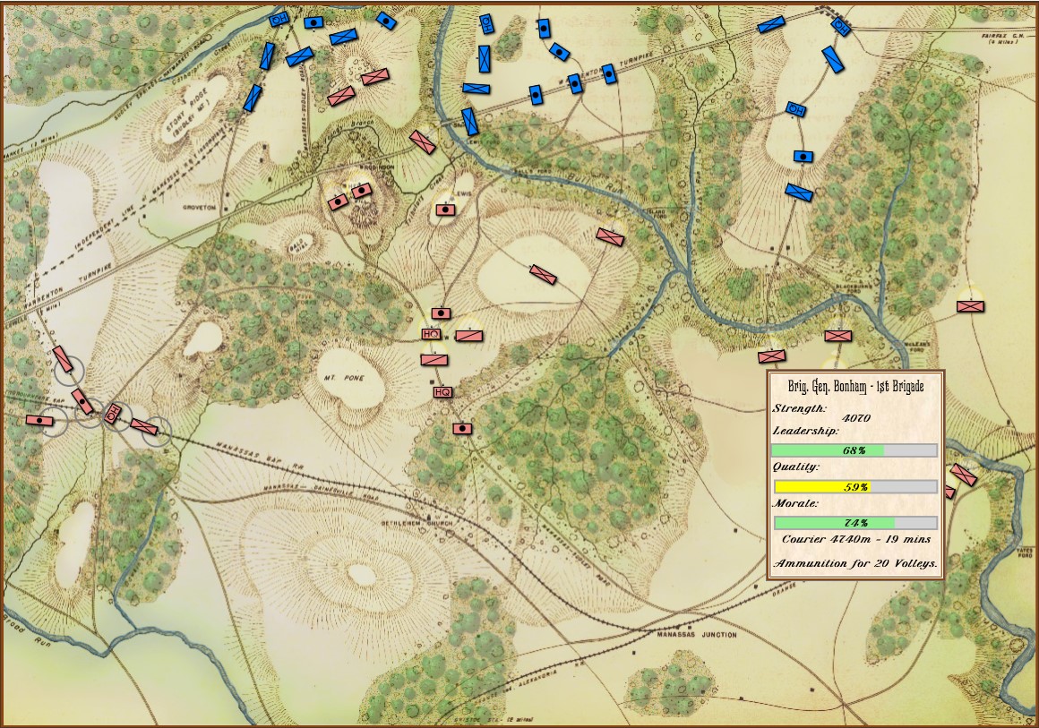
1st Bull Run, 11:30 AM, Simulation Mode, No Fog of War. Reinforcements shown. Click to enlarge.

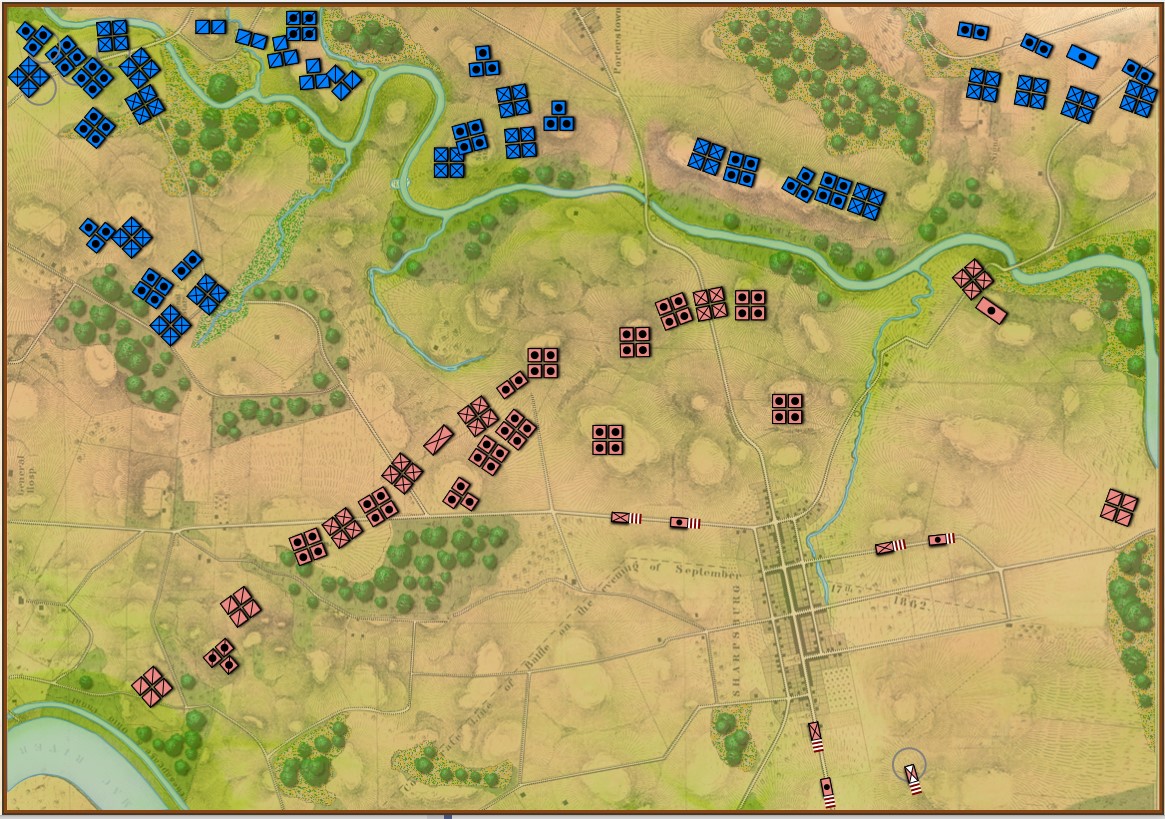
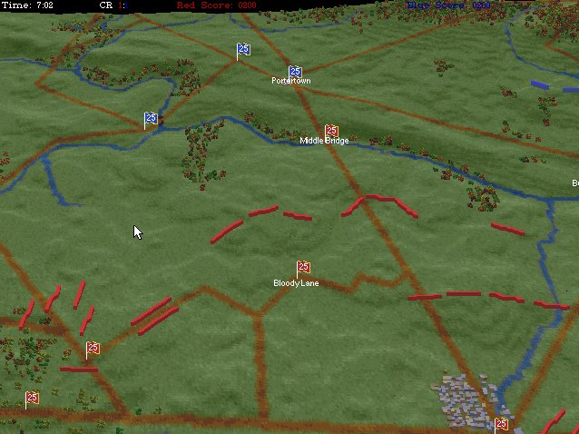
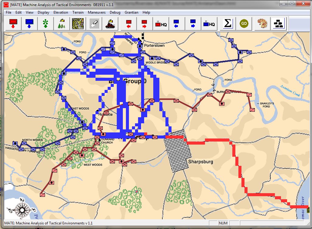
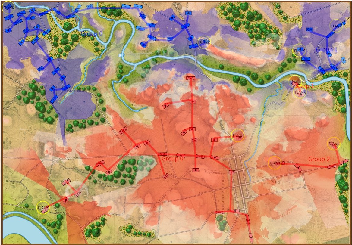
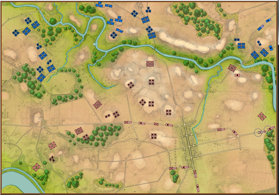
Antietam, 0600, Game Mode. Reinforcements shown. Click to enlarge.

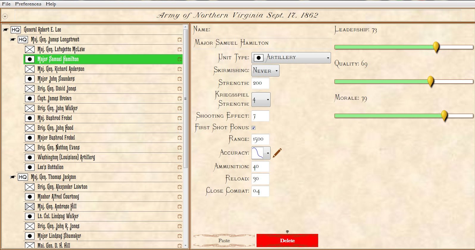
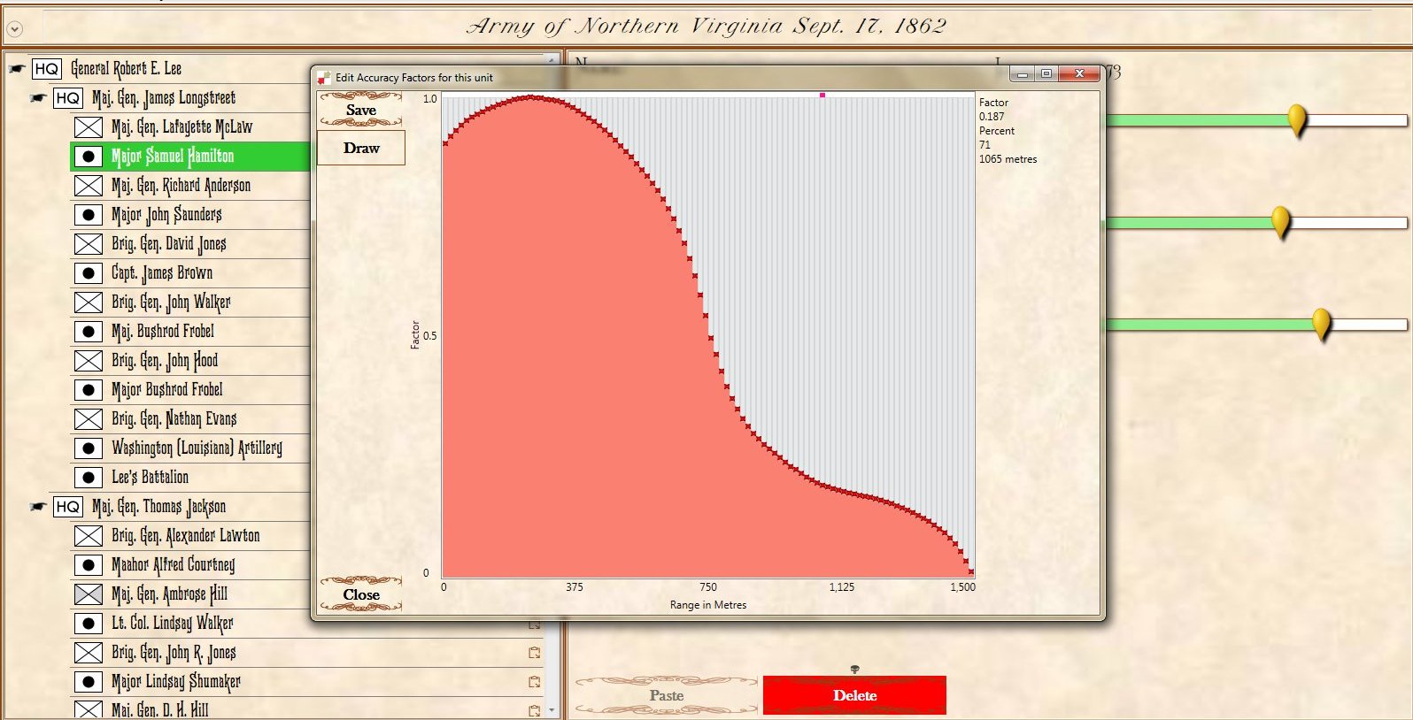
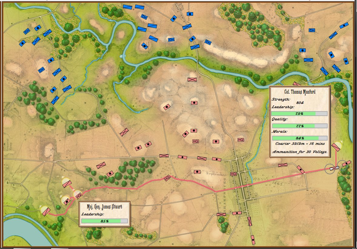
In the above two screen shots from General Staff you can clearly see the differences between Simulation and Game mode. In Simulation mode a unit’s exact strength in men, leadership value, morale value, experience value, number of volleys and the time it will take for a courier to travel from it’s commander’s HQ to the unit are displayed and tracked. In Game Mode, unit strength is represented by the number of icons (1 – 4) and leadership, morale, experience, and ammunition are not tracked. Units are moved directly by the player and there are no HQ units. In Simulation Mode, orders are given from the commanding HQ down to the subordinate commander’s HQ and then to the actual unit. The leadership value of each HQ effects how long the orders will be delayed on the way.

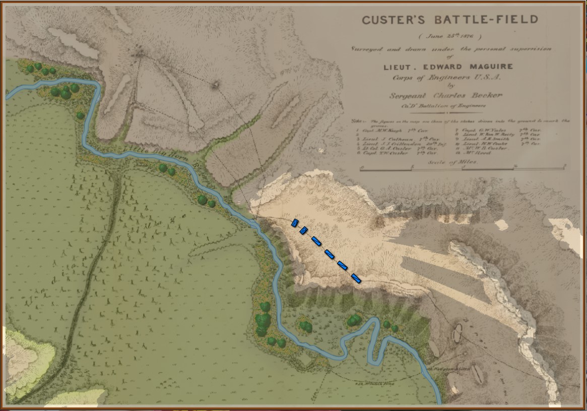
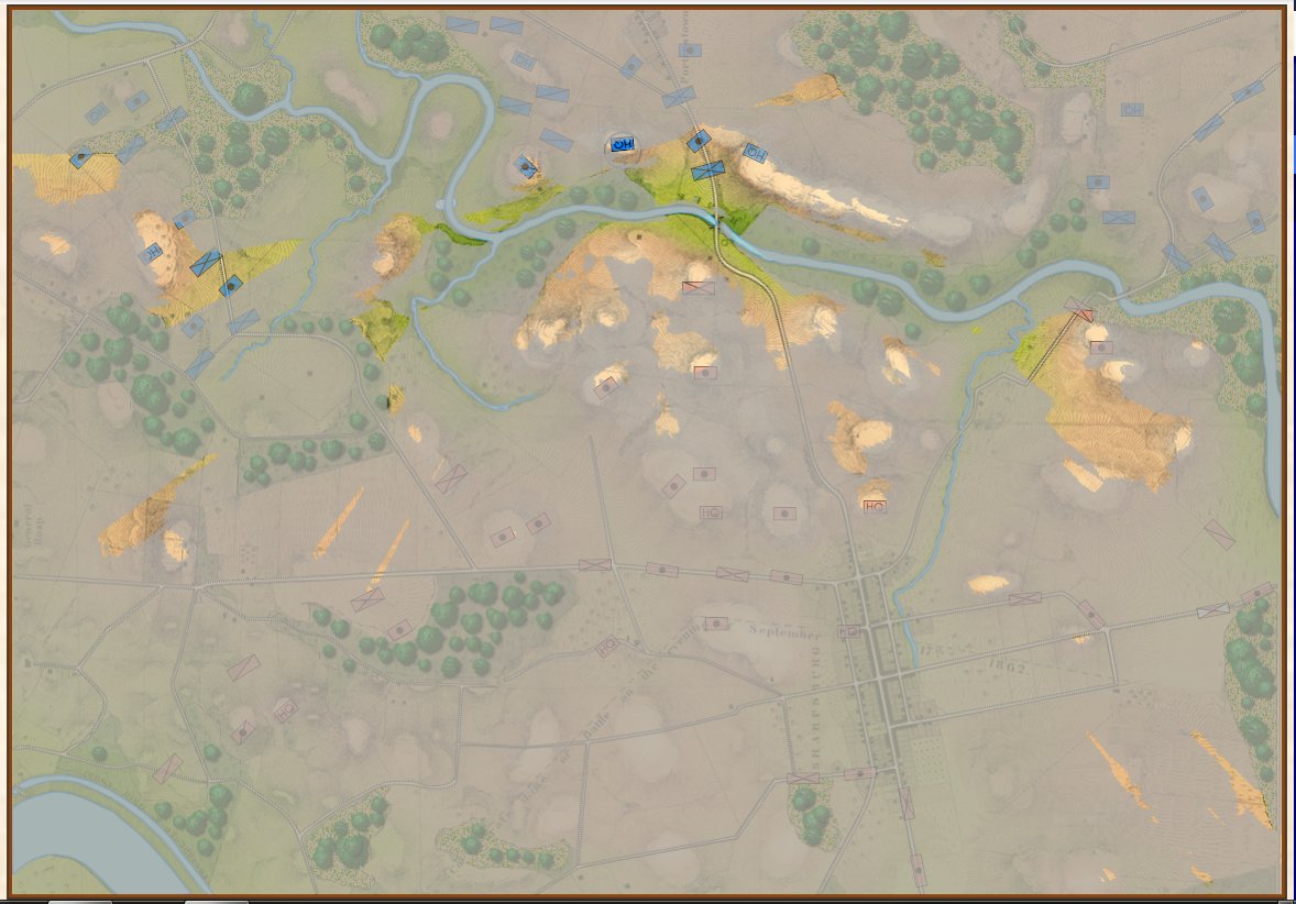
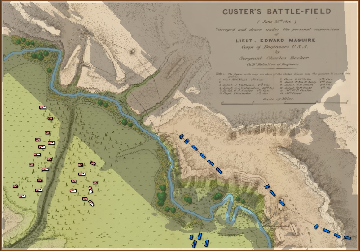
Little Bighorn, Simulation Mode, Complete Fog of War (from the commander’s perspective). Screen shot. Click to enlarge.

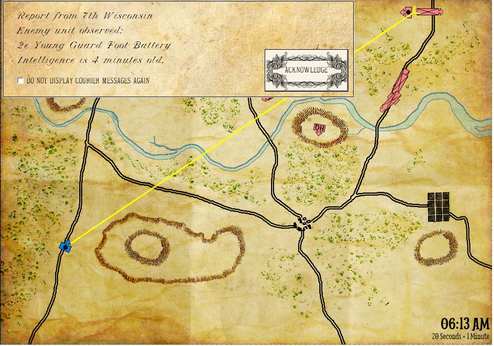
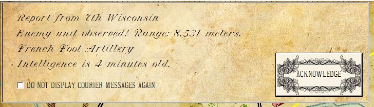
In the above screen shot, we see ‘Complete Fog of War’; only what the commander can see of the battlefield is displayed. In this case, this is what Colonel George Custer could see at this time. Just as in real life, in Complete Fog of War the commander receives dispatches from his troops about what they have observed; but this information is often stale and outdated by the time it arrives.

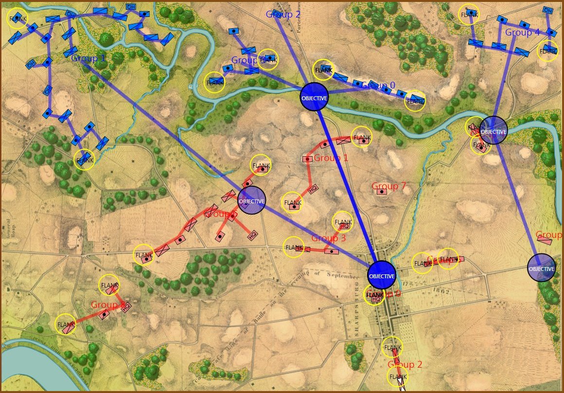
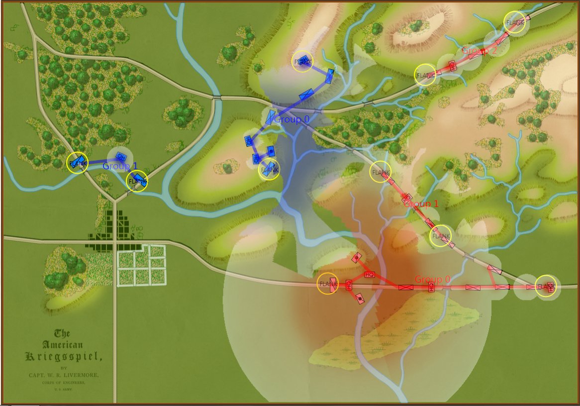
Little Bighorn, Simulation Mode, Partial Fog of War. This displays what all Blue forces can observe. Click to enlarge.

In the above screen shot Partial Fog of War is displayed. This is the sum of what is observable by all units (in this case, the Blue force). This is historically inaccurate for the 19th century and is included as an option because, frankly, users may want it and, programmatically, it was an easy feature to add. Throughout the development of General Staff we have consistently offered the users every conceivable option we can think of. That is also why we have included the option of, “No Fog o War,” with every unit visible on the battlefield. It’s an option and some users may want it.

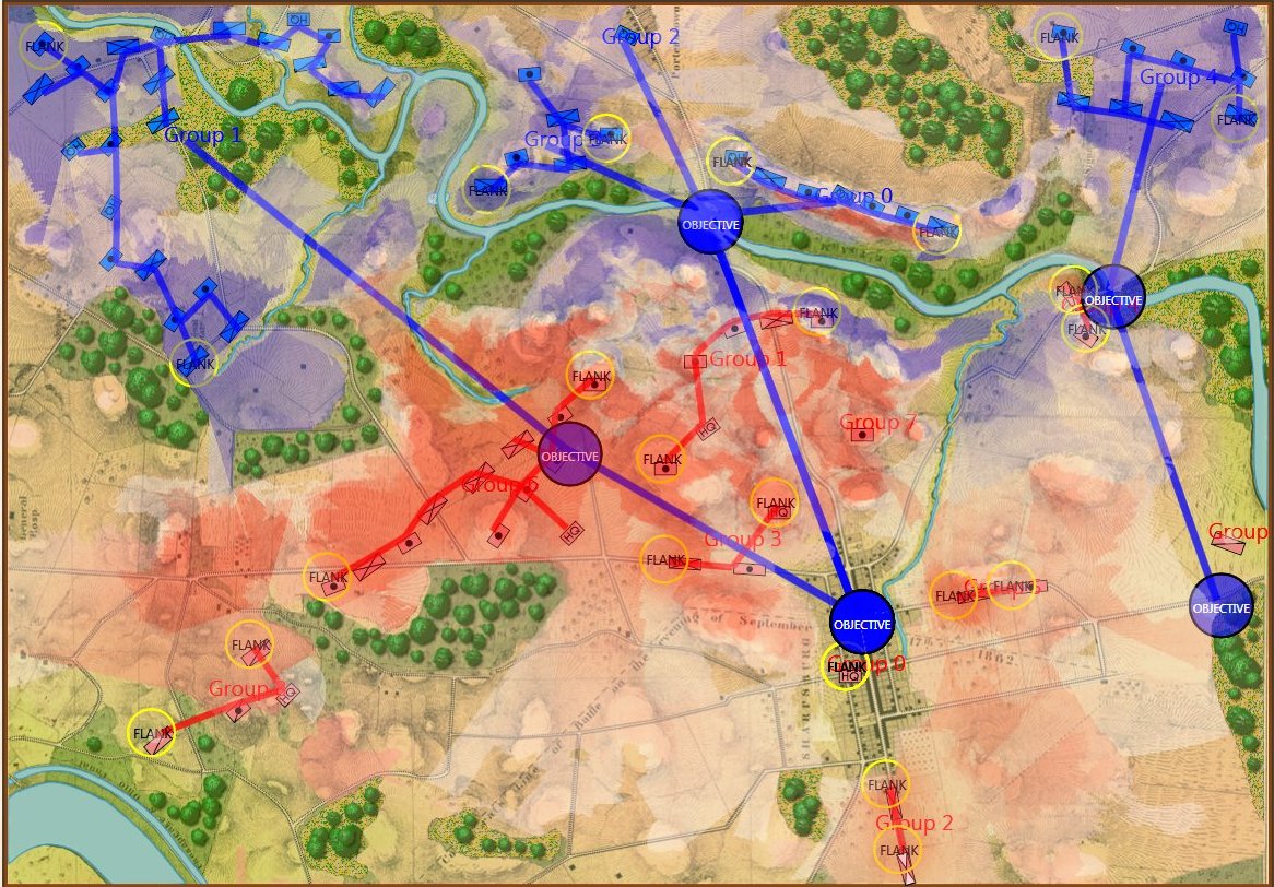
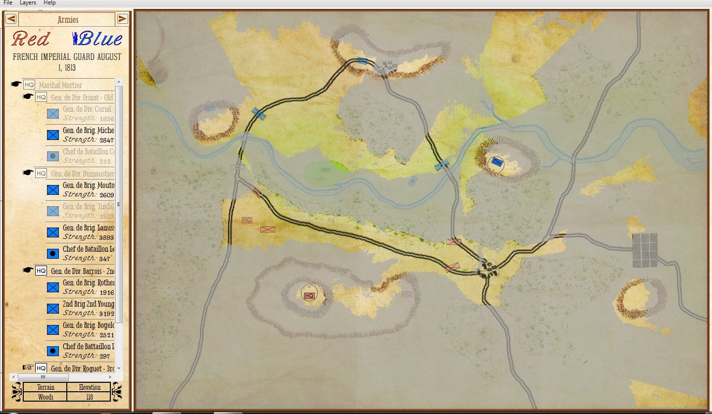
We have experimented with different ways of displaying ‘stale’ unit information including this method, below:

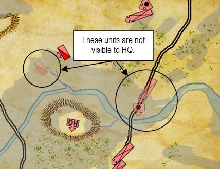
An example of how units that are not directly visible to HQ are displayed. The longer that a unit remains unobserved, the fainter it becomes. (Click to enlarge.)

We are now experimenting with overlays.

As always, your questions and comments are appreciated. Please feel free to email me directly.

Antietam & AI

6 Replies

MATE AI selected Objectives for Blue, 3D Line of Sight (3DLOS) and Range of Influence (ROI) displayed for the Antietam: Dawn General Staff scenario. Screen shot from General Staff Sand Box. Click to enlarge.

The author walking across Burnside’s Bridge in 1966 (age 12).

I have been thinking about creating an artificial intelligence (AI) that could make good tactical decisions for the battle of Antietam (September 17, 1862, Sharpsburg, Maryland) for over fifty years. At the time there was little thought of computers playing wargames.¹⁾However, it is important to note that Arthur Samuel had begun research in 1959 into a computer program that could play checkers. See. “Samuel, Arthur L. (1959). “Some Studies in Machine Learning Using the Game of Checkers”. IBM Journal of Research and Development.” What I was envisioning was a board wargame with some sort of look-up tables and coffee grinder slide rules that properly configured (not sure how, actually) would display what we now call a Course of Action (COA), or a set of tactical orders. I didn’t get too far on that project but I did create an Antietam board wargame when I was 13 though it was hardly capable of solitaire play.

The Antietam scenario from The War College (1992). This featured 128 pre-rendered 3D views generated from USGS Digital Elevation Model Maps.

In 1992 I created my first wargame with an Antietam scenario: The War College (above). It used a scripted AI that isn’t worth talking about. However, in 2003 when I began my doctoral research into tactical AI I had the firm goal in my mind of creating software that could ‘understand‘ the battle of Antietam.

TIGER Analysis of the battle of Antietam showing Range of Influence of both armies, battle lines and RED’s avenue of retreat. TIGER screen shot. Appears in doctoral thesis, “TIGER: A Machine Learning Tactical Inference Generator,” University of Iowa 2009

The TIGER program met that goal (the definition of ‘understand’ being: performing a tactical analysis that is statistically indistinguishable from a tactical analysis performed by 25 subject matter experts; e.g.. active duty command officers, professors of tactics at military institutes, etc.).

In the above screen shot we get a snapshot of how TIGER sees the battlefield. The darker the color the greater the firepower that one side or the other can train on that area. Also shown in the above screen shot is that RED has a very restricted Avenue of Retreat; the entire Confederate army would have to get across the Potomac using only one ford (that’s the red line tracing the road net to the Potomac). Note how overlapping ROIs cancel each other out. In my research I discovered that ROIs are very important for determining how battles are described. For example, some terms to describe tactical positions include:

Restricted Avenue of Attack
Restricted Avenue of Retreat
Anchored Flanks
Unanchored Flanks
Interior Lines
No Interior Lines

A Predicate Statement list generated by MATE for the battle of Antietam.

Between the time that I received my doctorate in computer science for this research and the time I became a Principal Investigator for DARPA on this project the name changed from TIGER to MATE (Machine Analysis of Tactical Environments) because DARPA already had a project named TIGER. MATE expanded on the TIGER AI research and added the concept of Predicate Statements. Each statement is a fact ascertained by the AI about the tactical situation on that battlefield. The most important statements appear in bold.

The key facts about the tactical situation at Antietam that MATE recognized were:

REDFOR’s flanks are anchored. There’s no point in attempting to turn the Confederate flanks because it can’t be done.
REDFOR has interior lines. Interior lines are in important tactical advantage. It allows Red to quickly shift troops from one side of the battlefield to the other while the attacker, Blue, has a much greater distance to travel.
REDFOR’s avenue of retreat is severely restricted. If Blue can capture the area that Red must traverse in a retreat, the entire Red army could be captured if defeated. Lee certainly was aware of this during the battle.
BLUEFOR’s avenue of attack is not restricted. Even though the Blue forces had two bridges (Middle Bridge and Burnside’s Bridge) before them, MATE determined that Blue had the option of a wide maneuver to the north and then west to attack Red (see below screen shot):

MATE analysis shows that Blue units are not restricted to just the two bridge crossings to attack Red. MATE screen shot.

BLUEFOR has the superior force. The Union army was certainly larger in men and materiel at Antietam.
BLUEFOR is attacking across level ground. Blue is not looking at storming a ridge like at the battle of Fredericksburg.

MATE AI selects these objectives for Blue’s attack. General Staff Sand Box screen shot. Click to enlarge.

We now come to General Staff which uses the MATE AI. General Staff clearly has a much higher resolution than the original TIGER program (1155 x 805 terrain / elevation data points versus 102 x 66, or approximately 138 times the resolution / detail). In the above screen shot the AI has selected five Objectives for Blue. I’ve added the concept of a ‘battle group’ – units that share a contiguous battle line – which in this case works out as one or two corps. Each battle group has been assigned an objective. How each battle group achieves its objective is determined by research that I did earlier on offensive tactical maneuvers ²⁾See, “Implementing the Five Canonical Offensive Maneuvers in a CGF Environment.” link to paper.

As always, I appreciate comments and questions. Please feel free to email me directly with either.

References[+]

References
↑1	However, it is important to note that Arthur Samuel had begun research in 1959 into a computer program that could play checkers. See. “Samuel, Arthur L. (1959). “Some Studies in Machine Learning Using the Game of Checkers”. IBM Journal of Research and Development.”
↑2	See, “Implementing the Five Canonical Offensive Maneuvers in a CGF Environment.” link to paper.

Wargame AI Continued: Range of Influence

4 Replies

In two previous blogs I wrote about how Artificial Intelligence (AI) for wargames perceive battle lines and terrain and elevation. Today the topic is how computer AI has changed ‘Range of Influence’ (ROI) or ‘Zone of Control’ (ZOC) analysis. Range of Influence and Zone of Control are terms that can be used interchangeably. Basically, what they mean is, “how far can this unit project its power.”

One of the first appearances of range as a wargame variable was in Livermore’s 1882 American Kriegsspiel: A Game for Practicing the Art of War Upon a Topographical Map (superb article on American Kriegsspiel here). Note that incorporated into the ‘range ruler’ (below) is also a linear ‘effectiveness scale’.

Detail of Plate IV, “The Firing Board,” from the American Kriegsspil showing a ruler for artillery range printed on the top. Note the accuracy declines (apparently linearly) proportional to the distance. Click to enlarge.

The introduction of hexagon wargames (first at RAND and then later by Roberts at Avalon Hill; see here) created the now familiar 6 hexagon ‘ring’ for a Zone of Control:

Zone of Control explained in the Avalon Hill Waterloo (1962) manual. Author’s Collection.

I seem to remember an Avalon Hill game where artillery had a 2 hex range; but I may well be mistaken.

Ever since the first computer wargames that I wrote back in the ’80s I have earnestly tried to make the simulations as accurate as possible by including every reasonable variable. With the General Staff Wargaming System we’ve added two new variables to ROI: 3D Line of Sight and an Accuracy curve.

Order of Battle for Antietam showing Hamilton’s battery being edited. Screen shot from the General Staff Army Editor. Click to enlarge.

In the above image we are editing a Confederate battery in Longstreet’s corps. Every unit can have a unique unit range and accuracy. You can select an accuracy curve from the drop-down menu or you can create a custom accuracy curve by clicking on the pencil (Edit) icon.

Window for editing the artillery accuracy curve. There are 100 points and you can set each one individually. This also supports a digitizing pen and drawing tablet. Screen shot from General Staff Army Editor. Click to enlarge.

In the above screen shot from the General Staff Wargaming System Army Editor the accuracy curve for this particular battery is being edited. There are 100 points that can be edited. As you move across the curve the accuracy at the range is displayed in the upper right hand corner. Note: every unit in the General Staff Wargaming System can have a unique accuracy curve as well as range and every other variable.

Screen shot showing the Range of Influence fields for a scenario from the 1882 American Kriegsspiel book. Click to enlarge.

In the above screen shot from the General Staff Sand Box (which is used to test AI and combat) we see the ROI for a rear guard scenario from the original American Kriegsspiel 1882. Notice that the southern-most Red Horse Artillery unit has a mostly unobstructed field of vision and you can clearly see how accuracy diminishes as range increases. Also, notice how the ROI for the one Blue Horse Artillery unit is restricted by the woods which obstructs its line of sight.

Screen shot of Antietam (dawn) showing Red and Blue ROI and battle lines. Click to enlarge.

In the above screen shot we see the situation at Antietam at dawn. Blue and Red units are rushing on to the field and establishing battle lines. Again, notice how terrain and elevation effects ROI. In the above screen shot Blue artillery’s ROI is restricted by the North Woods.

The above ROI maps (screen shots) were created by the General Staff Sand Box program to visually ‘debug’ the ROI (confirm that it’s working properly). We probably won’t include this feature in the actual General Staff Wargame unless users would like to see it added.

This is a topic that is very near and dear to my heart. Please feel free to contact me directly if you have any questions or comments.

How Will You Play General Staff?

32 Replies

Every wargame that I’ve designed allows the user to adjust important variables such as leadership and morale and how they affect combat. Usually included is the ability to design your own armies, maps and scenarios as well. However, with the General Staff Wargaming System we’ve added a new feature: the ability to control the realism level before playing a scenario.

The General Staff Wargame has two basic levels of play:

Simulation mode uses HQ units and a chain of command that passes orders down from the General HQ to the sub-commander to the individual unit. How fast the unit responds to the orders are affected by the distance that the courier must travel and the Leadership Value of the HQs. Simulation mode also employs a more detailed combat resolution model and tracks the actual number of troops in every unit.

An example of Simulation Mode: the path (red line) and time (16 minutes) it will take for a courier to travel from JEB Stuart’s HQ to Munford’s cavalry with orders. Click to enlarge.

Kriegsspiel mode does not have HQ units and friendly units are moved directly and immediately (no transmission of orders via couriers). The combat resolution model is simpler and units have a value of 1-4 displayed by the number of unit icons on the map.

Antietam in Kriegsspiel mode. Notice that there are no HQ units (so no couriers to deliver orders) and units are represented by 1-4 icons. Units in column have a ‘tail’ that indicates the unit strength. Click to enlarge.

In addition to the two game modes (Simulation and Kriegsspiel) there are three Scenario Options:

Order of Battle (OOB) displayed / not displayed. Enemy units with known positions appear dark; enemy units ‘on the map’ but with unknown locations appear grayed out. This, of course, gives the user complete knowledge of the enemy’s OOB and, more importantly, knows when units from certain formations are not directly observable.

A mock up of how the Order of Battle option will appear (note this image was created from screen captures of the Scenario Editor and the Sand Box). Click to enlarge

Only friendly units directly observed by the General HQ are displayed. All other friendly units fade at their last known location. Couriers bring in unit location updates, but they are outdated by the time they arrive.

Only enemy units directly observed by the General HQ are displayed. All other enemy units fade at their last known location. Couriers bring in unit location updates, but they are outdated by the time they arrive.

If both of these above options are selected (only friendly and enemy units that are directly observable by your commanding General HQ) you will be simulating the Fog of War that field commanders of the age of gunpowder experienced.

What General George B. McClellan could actually see at Antietam. Screen shot (General Staff Sand Box). Click to enlarge.

We would like to hear from you and get your opinion on what realism features you will use in General Staff:

The Fog of War

10 Replies

A key element of General Staff gameplay is the notion of ‘fog of war’. In essence we keep three maps: what blue thinks the situation is, what red thinks the situation is and where all units actually are on the map.

A courier reports that an enemy unit was observed four minutes ago. Note: the enemy unit has almost certainly moved on since then. (Click to enlarge.)

Location of your headquarters (HQ) unit is vitally important in General Staff. If an enemy (or friendly) unit is not directly observable to your HQ unit, the information of an enemy unit sighting is passed to HQ via courier. The amount of time for the courier to travel from the observing unit to the HQ is precisely calculated (see screen capture, above). Friendly units report their position every hour and dispatch a courier to HQ with this information as well. The time for a courier to travel from the reporting unit to travel to HQ is also calculated.

In essence, then, locating your HQ unit on a hill, ridge or other prominent feature is important if you want a clear view of the battlefield. Otherwise, you will be dependent on your couriers to penetrate the fog of war.

The phrase, ‘Fog of War’ (or Nebel des Krieges in German) was first written by Carl von Clauswitz in his famous treatise, On War (in 1832, first English translation in 1873):

War is the realm of uncertainty; three quarters of the factors on which action in war is based are wrapped in a fog of greater or lesser uncertainty. A sensitive and discriminating judgment is called for; a skilled intelligence to scent out the truth.

— Carl von Clausewitz

Update: some readers at Kriegsspiel Forum have quite correctly pointed out that at great distances units would certainly not be able to ascertain the name of the unit that they are observing. Consequently, we have changed the information provided to this:

Dispatch from observing unit modified to include distance and just unit type. (Click to enlarge.)

Now the question arises: how far could you see with a 19th century telescope? Do we need to include a maximum range for line of sight? Interesting question. Would like to hear your comments.