Category Archives: Computers

Wargame AI Continued: Range of Influence

In two previous blogs I wrote about how Artificial Intelligence (AI) for wargames perceive battle lines and terrain and elevation. Today the topic is how computer AI has changed ‘Range of Influence’  (ROI) or ‘Zone of Control’ (ZOC) analysis. Range of Influence  and Zone of Control are terms that can be used interchangeably. Basically, what they mean is, “how far can this unit project its power.”

One of the first appearances of range as a wargame variable was in Livermore’s 1882 American Kriegsspiel: A Game for Practicing the Art of War Upon a Topographical Map (superb article on American Kriegsspiel here).  Note that incorporated into the ‘range ruler’ (below) is also a linear ‘effectiveness scale’.

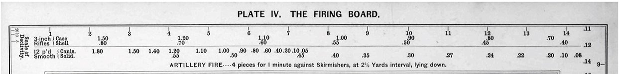
Detail of Plate IV, “The Firing Board,” from the American Kriegsspil showing a ruler for artillery range printed on the top. Note the accuracy declines (apparently linearly) proportional to the distance. Click to enlarge.

The introduction of hexagon wargames (first at RAND and then later by Roberts at Avalon Hill; see here) created the now familiar 6 hexagon ‘ring’ for a Zone of Control:

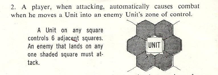
Zone of Control explained in the Avalon Hill Waterloo (1962) manual. Author’s Collection.

I seem to remember an Avalon Hill game where artillery had a 2 hex range; but I may well be mistaken.

Ever since the first computer wargames that I wrote back in the ’80s I have earnestly tried to make the simulations as accurate as possible by including every reasonable variable. With the General Staff Wargaming System we’ve added two new variables to ROI: 3D Line of Sight and an Accuracy curve.

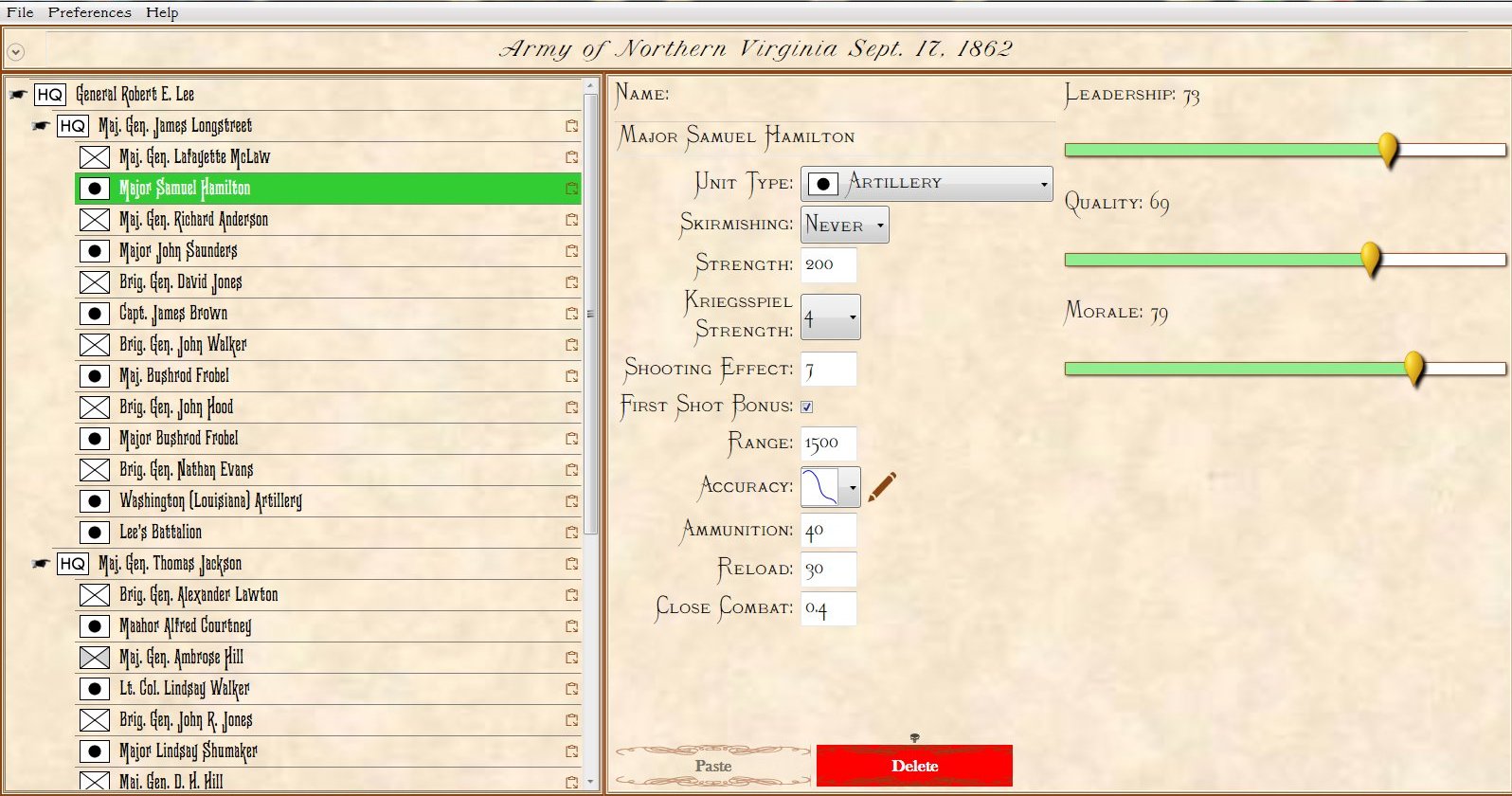
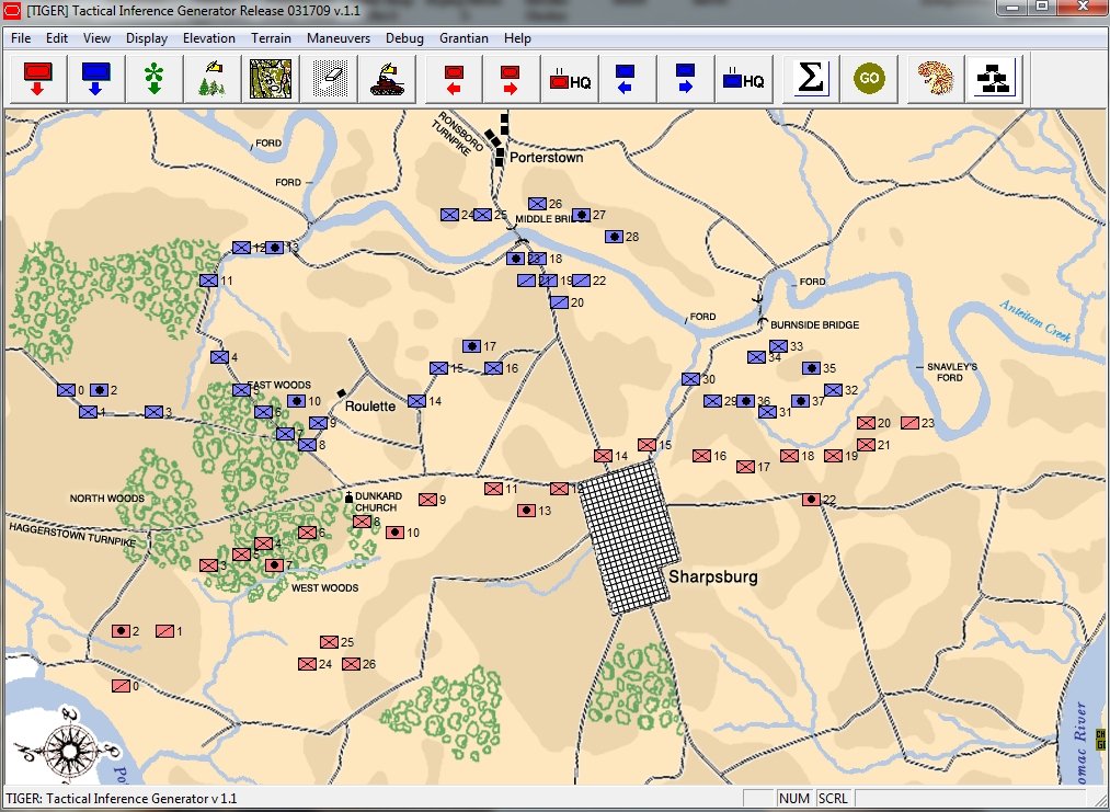
Order of Battle for Antietam showing Hamilton’s battery being edited. Screen shot from the General Staff Army Editor. Click to enlarge.

In the above image we are editing a Confederate battery in Longstreet’s corps. Every unit can have a unique unit range and accuracy. You can select an accuracy curve from the drop-down menu or you can create a custom accuracy curve by clicking on the pencil (Edit) icon.

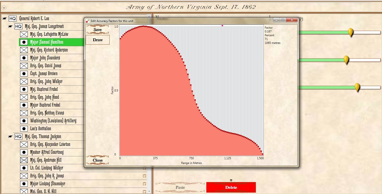
Window for editing the artillery accuracy curve. There are 100 points and you can set each one individually. This also supports a digitizing pen and drawing tablet. Screen shot from General Staff Army Editor. Click to enlarge.

In the above screen shot from the General Staff Wargaming System Army Editor the accuracy curve for this particular battery is being edited. There are 100 points that can be edited. As you move across the curve the accuracy at the range is displayed in the upper right hand corner. Note: every unit in the General Staff Wargaming System can have a unique accuracy curve as well as range and every other variable.

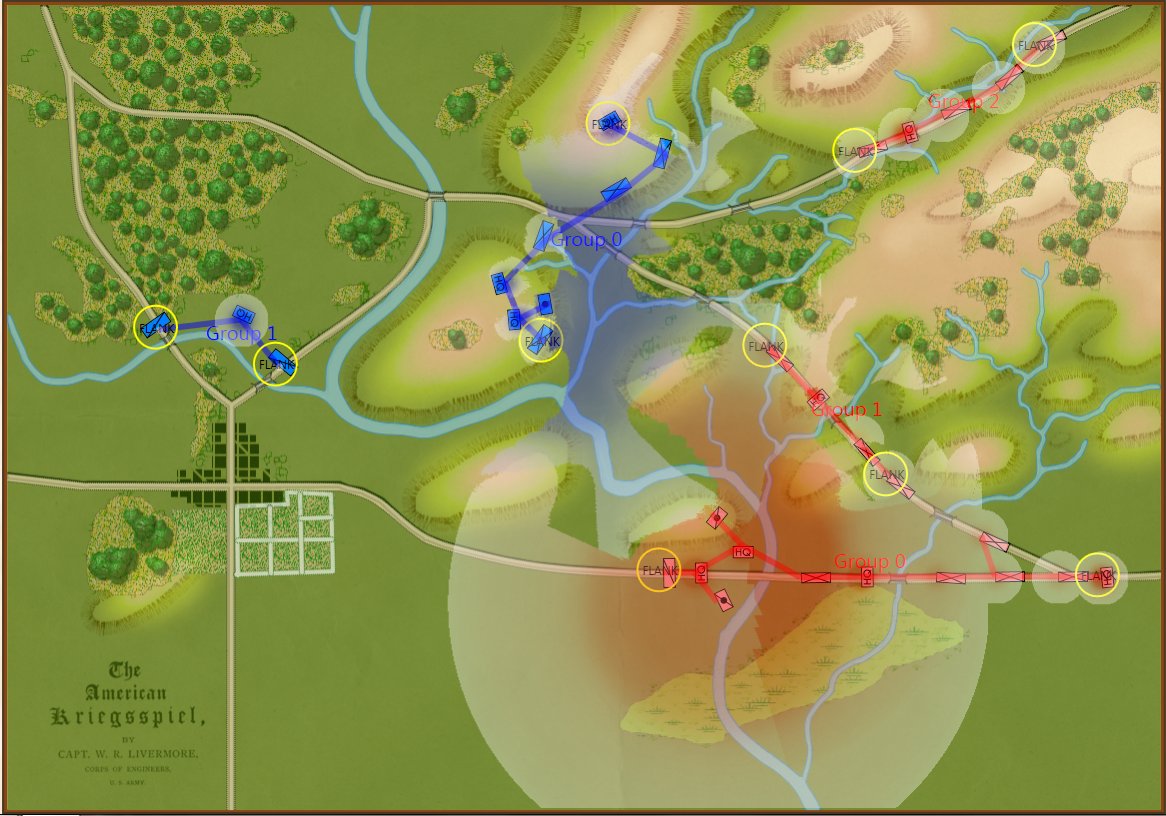
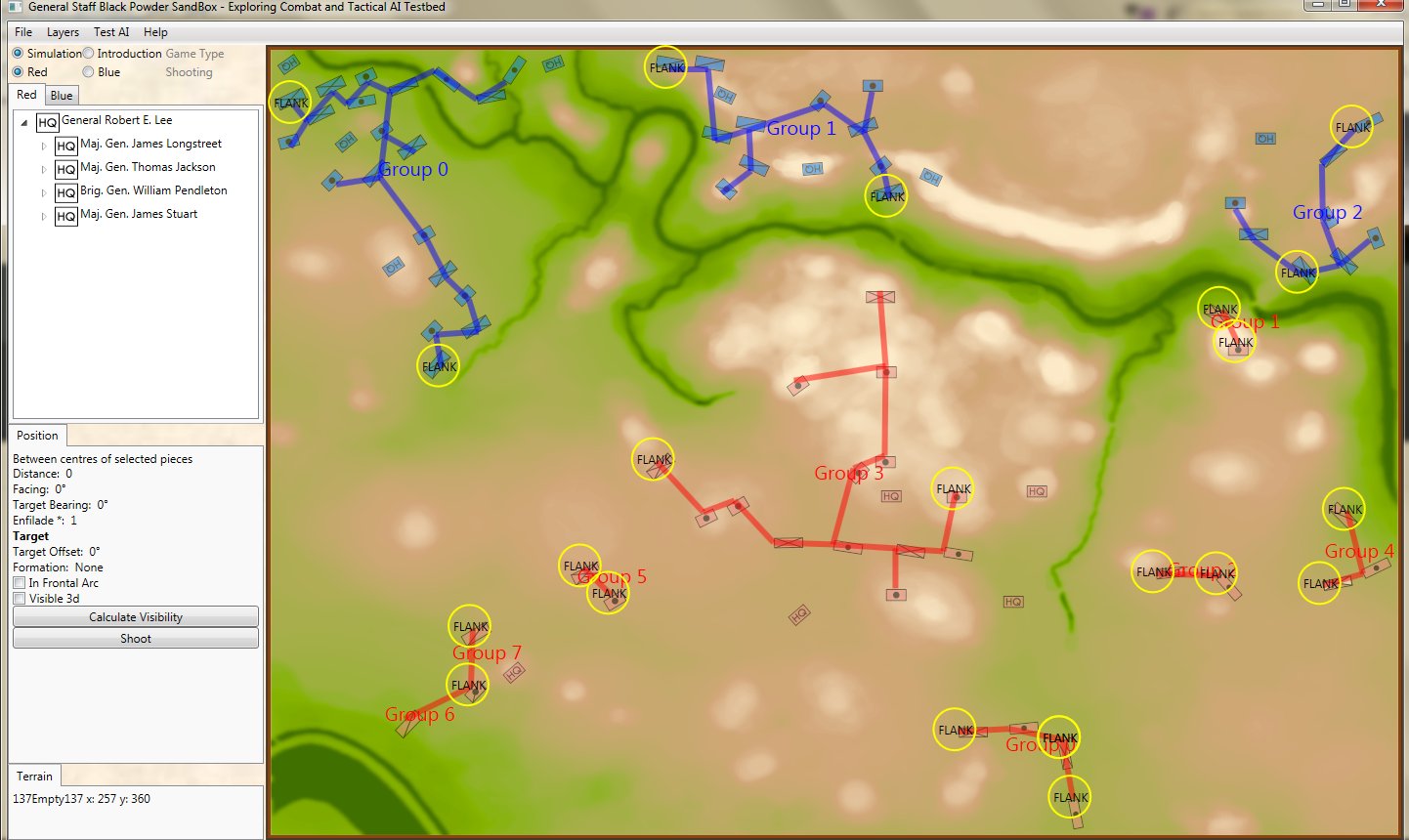
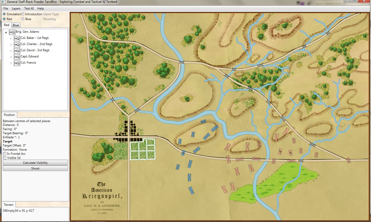
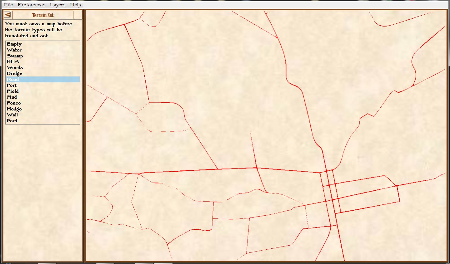
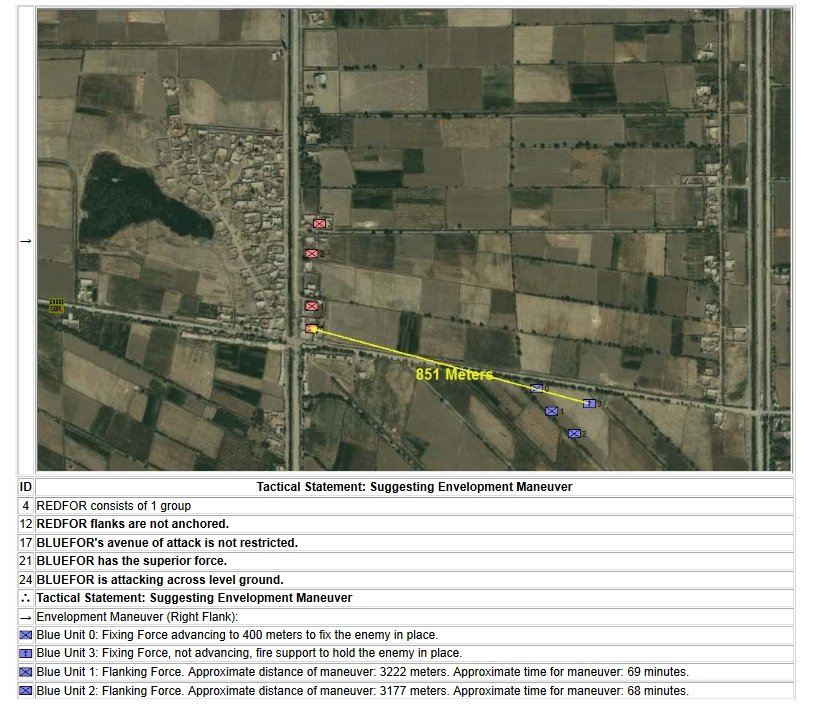
Screen shot showing the Range of Influence fields for a scenario from the 1882 American Kriegsspiel book. Click to enlarge.

In the above screen shot from the General Staff Sand Box (which is used to test AI and combat) we see the ROI for a rear guard scenario from the original American Kriegsspiel 1882. Notice that the southern-most Red Horse Artillery unit has a mostly unobstructed field of vision and you can clearly see how accuracy diminishes as range increases. Also, notice how the ROI for the one Blue Horse Artillery unit is restricted by the woods which obstructs its line of sight.

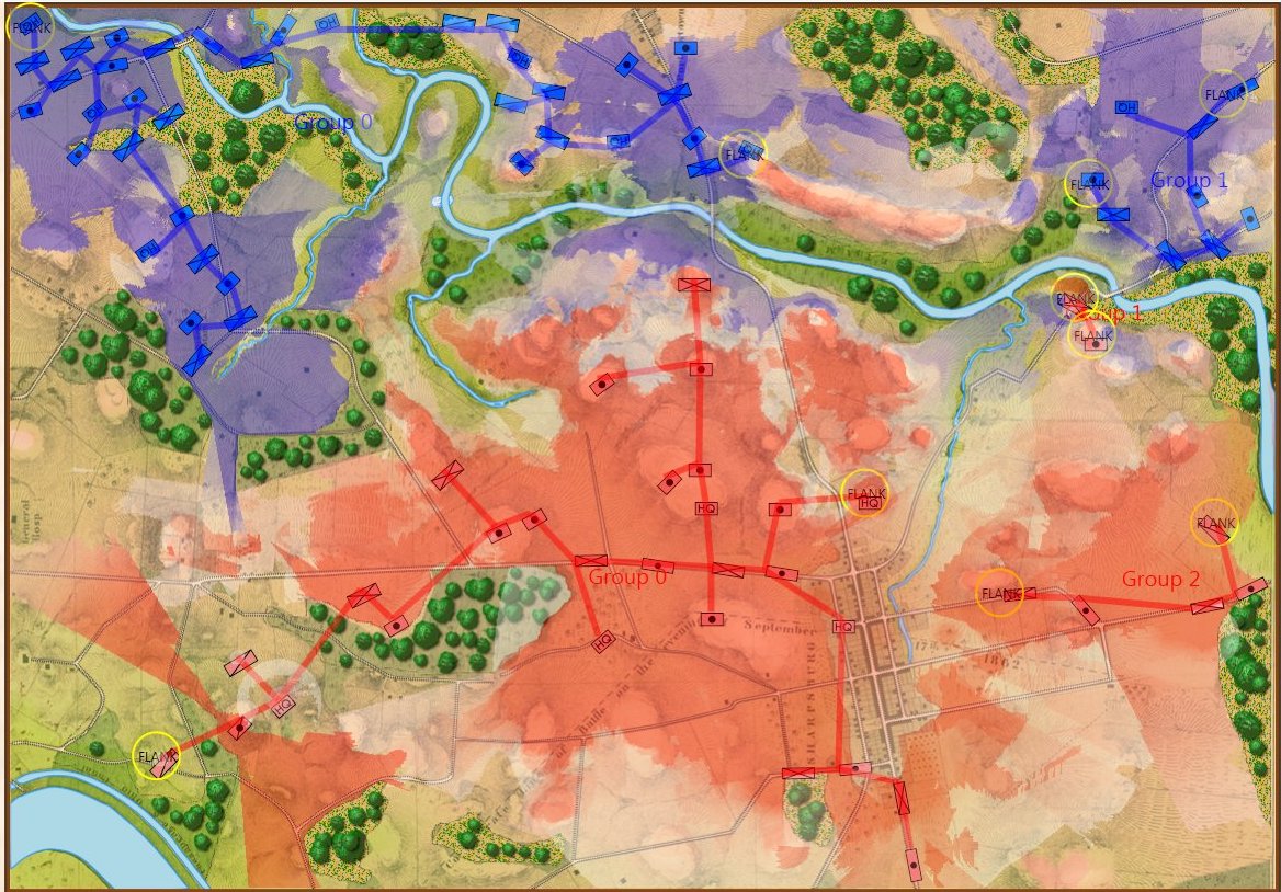
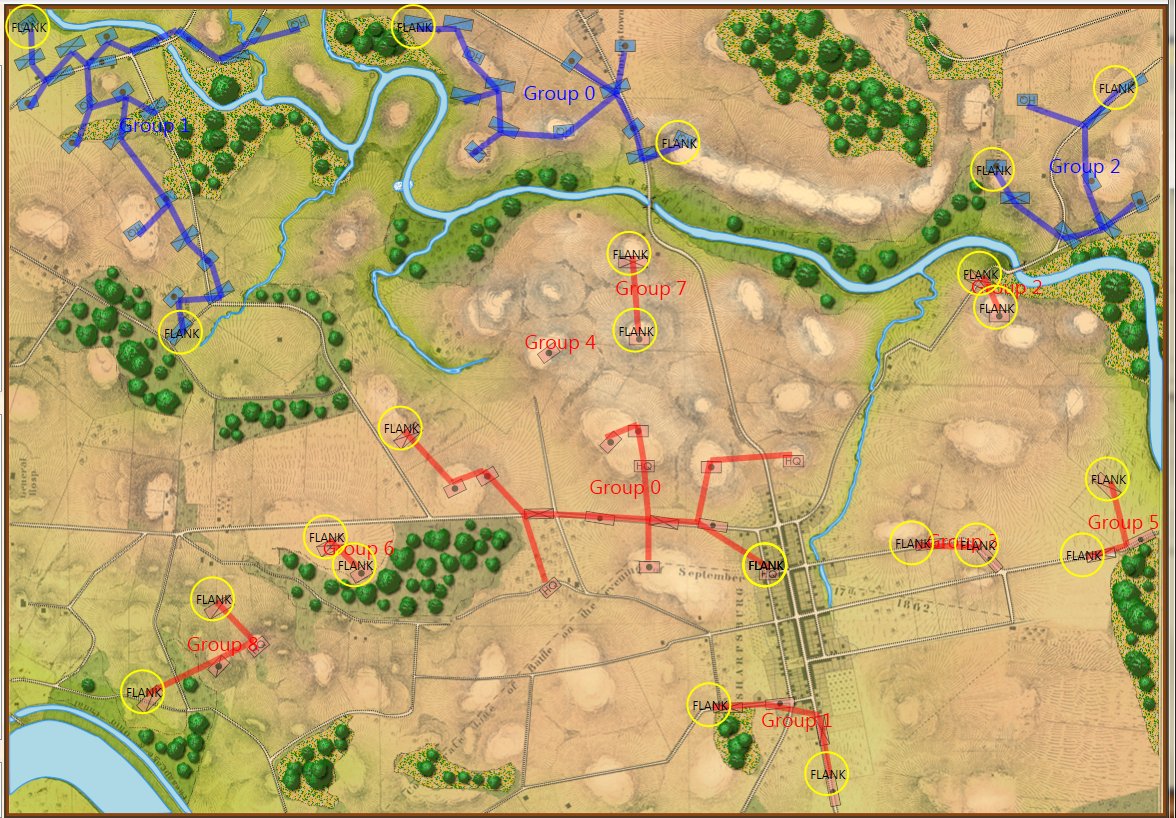
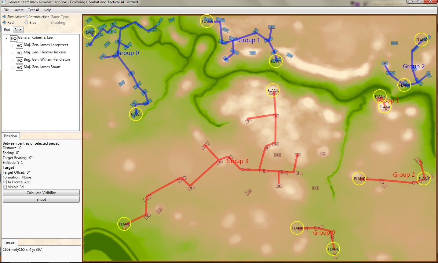
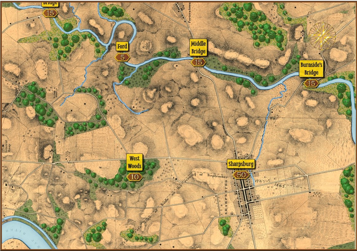
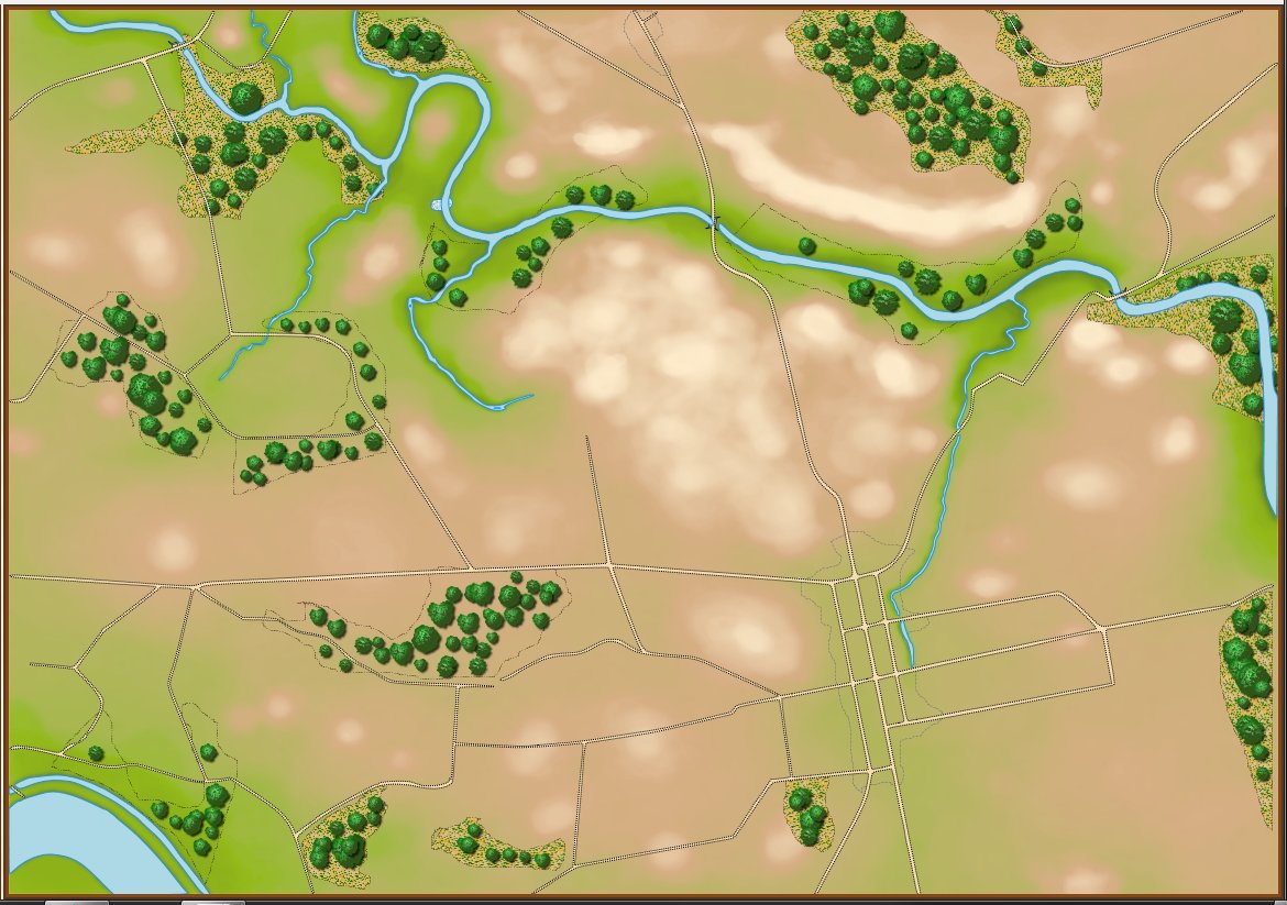
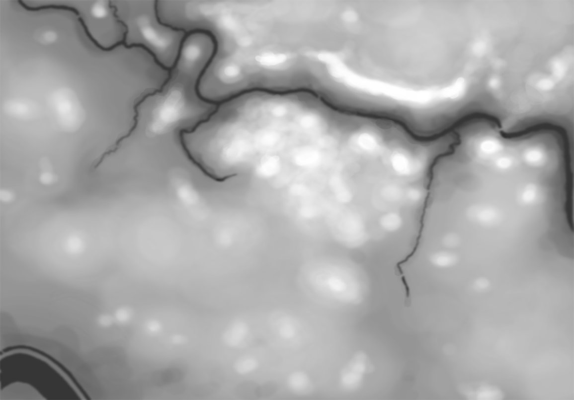
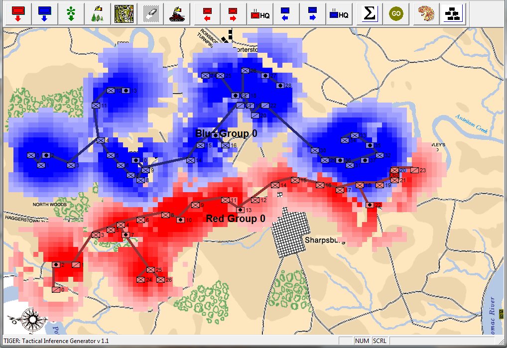
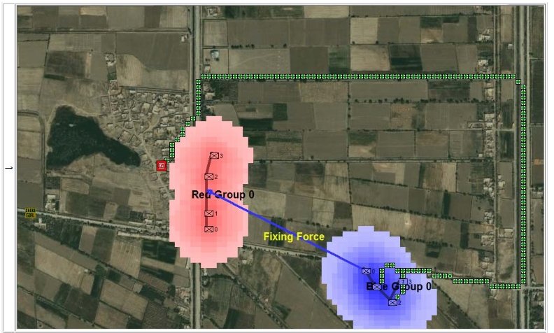
Screen shot of Antietam (dawn) showing Red and Blue ROI and battle lines. Click to enlarge.

In the above screen shot we see the situation at Antietam at dawn. Blue and Red units are rushing on to the field and establishing battle lines. Again, notice how terrain and elevation effects ROI. In the above screen shot Blue artillery’s ROI is restricted by the North Woods.

The above ROI maps (screen shots) were created by the General Staff Sand Box program to visually ‘debug’ the ROI (confirm that it’s working properly). We probably won’t include this feature in the actual General Staff Wargame unless users would like to see it added.

This is a topic that is very near and dear to my heart. Please feel free to contact me directly if you have any questions or comments.

What’s Wrong With This Picture?

Computer AI representation of battle lines for Antietam, dawn September 17, 1862. The AI is locating the Schwerpunkt or place to attack. Click to enlarge.

I was looking at this screen shot I posted as an illustration in my blog post, Battle Lines, Commanders & Computers (link) and something didn’t look right. Specifically, it was the Flank markers for Stewart’s cavalry on the Confederate left flank. And, the more I looked, the more I noticed other problems: Stewart’s cavalry was captioned as being in two groups (Group 6 and Group 7). There was an extra Flank marker with the Confederate reinforcements entering the field at the bottom of the map, the Flank markers for Union Group 2 were clearly wrong, too.

This began a two week long bug hunt that took me places I didn’t expect to revisit. To make a long story short – and how often have you heard that phrase but this is actually one of those few occasions when it’s true – I had to go back and look at my original computer code that I wrote in grad school and it turns out that there was a ‘worst case’ bug that just happened to pop up with the Antietam scenario.

This is what the battle lines and Flank markers should really look like (note: the map layer is turned on here and you can’t see the elevation layer like the top screen shot):

Correct battle lines and Flank markers for the battle of Antietam. Screen shot from the General Staff Sand Box AI test program. Click to enlarge.

I also discovered a logic flaw – a mental bug, if you will – in my definition of Flank units. Previously, I defined them as as the ‘maximally separated units of a MST (battle line) group’. That seems correct but if you think about it there are rare circumstances when this is not correct (think of the horseshoe lines at Gettysburg for example). I changed the definition of Flank units to: the ‘maximally separated units of a MST group with only one neighbor (i.e. they are at the end of a battle line and, therefore, have only one neighbor).

I thought I would finish this blog post with something that is truly unique: the very first computer bug:

On September 9, 1947 Grace Murray Hopper records ‘the first computer bug’ in the Harvard Mark II computer’s log book. Apparently, the moth was caught in a relay switch. And, yes, this is where the term comes from. Click to enlarge.


Battle Lines, Commanders & Computers

When we look at maps of battles even the novice armchair general can quickly trace the battle lines of the armies. Recognizing battle lines is one of the most important skills a commander – or a wargaming Artificial Intelligence (AI) – can possess. Without this ability how will you identify the flanking units? And if you can’t identify the units at the end of a line, how will you implement a flanking attack around them? Equally important is the ability to identify weak points in a battle line.

The algorithm for detecting battle lines and flank units is one of the ‘building block’ algorithms of my TIGER / MATE tactical AI and first appeared in my paper, Implementing the Five Canonical Offensive Maneuvers in a CGI Environment1)http://riverviewai.com/papers/ImplementingManeuvers.pdf. I will discuss how the algorithm works at the end of this blog. For now, just accept that it finds lines and flanks.

Let’s look at some examples of the General Staff AI ‘parsing’ unit positions. First, the battle of Antietam, situation at dawn (by the way, Antietam is one of the free scenarios included with the General Staff Wargaming System):

The battle of Antietam, dawn, September 17, 1863. Screen shot from the General Staff Sand Box program. Click to enlarge.

This is how a human sees the tactical situation: units on a topographical map. But, the computer AI sees it quite differently. In the next image, below, the battle lines and elevation are displayed as the AI sees the battle (note: the AI also ‘sees’ the terrain but, for clarity, that is not being shown in this screen capture):

The battle of Antietam, September 17, 1862 dawn, with computer AI battle lines and elevation displayed. Note: the identification of flank units. Both red and blue forces are assembling on the field. Click to enlarge.

What is immediately obvious is that Red (Confederate) forces are hastily constructing a battle line while Blue (Union) forces are beginning to pour onto the battlefield to attack.  Let us now ask the question: what is the weakest point of the Red battle line? Where should Blue attack? This point is sometimes called the Schwerpunkt. German for point of maximum effort2)See also, “Clausewitz’s Schwerpunkt Mistranslated from German, Misunderstood in English” Military Review, 2007 https://www.armyupress.army.mil/Portals/7/military-review/Archives/English/MilitaryReview_20070228_art014.pdf. Where should Blue concentrate its forces?

Computer AI representation of battle lines for Antietam, dawn September 17, 1862. The AI is locating the Schwerpunkt or place to attack. Click to enlarge.

Now that the weakest points of Red’s battle line have been identified, Blue (assuming Blue is being controlled by the AI) can exploit it by attacking the gaps in Red’s battle line. The Blue AI can order either a Penetration or Infiltration Maneuver to exploit these gaps (the following images are from my paper, “Implementing the Five Canonical Offensive Maneuvers in a CGF Environment.” Note, in the TIGER / MATE screen shots below Range of Influence (ROI) is also visible:

From the paper, “Implementing the Five Canonical Offensive Maneuvers.”

Both of these maneuvers are possible because the AI has identified weak points in the OPFOR (Opponent Forces) battle lines. Equally important when discussing battle lines are the location of the flanks. The next two images use the original American Kriegsspiel (1882) map which is also included in the General Staff Wargaming System:

The original American Kriegsspiel map (1882) restored and now used in the General Staff Wargaming System. Screen shot from the General Staff Sand Box AI test program. Click to enlarge.

In this screen capture from the General Staff Wargaming System Sand Box AI test program battle lines are displayed by the AI. Note the flank units and especially the unanchored (or open) Blue flank. Click to enlarge.

Identifying flank units is vitally important in the Turning Maneuver and the Envelopment Maneuver:

Knowing the location of flank units is also important for classifying tactical positions (this will be the subject of an upcoming blog).

So, how does this algorithm work?

I’ve never been a fan of graph theory; or heavy mathematical lifting in general. One of the required classes in grad school was Design and Analysis of Algorithms and it got into graph theory quite a bit. The whole time I was thinking, “I’m never going to use any of this stuff, but I have to get at least a B+ to graduate,” so I took a lot of notes and studied hard. Later, when I was looking for a framework to understand tactics and to write a tactical AI it became obvious that graph theory was at least part of the solution. Maps are routinely divided into a grid, unit locations can be points (or vertices) at the intersections of these lines. Battle lines can be edges that connect the vertices. I need to publicly thank my doctoral advisor, Dr. Alberto Segre, for first suggesting that battle lines could be described using something called a Minimum Spanning Tree3)https://en.wikipedia.org/wiki/Minimum_spanning_tree (MST). An MST is the minimum possible distances (edge weights to be precise) to connect all the vertices in a tree (or a group, as I call them in the above screen shots).

I ended up implementing Kruskal’s algorithm4)https://en.wikipedia.org/wiki/Kruskal’s_algorithm for identifying battle lines. It is what is called a ‘greedy algorithm’ and it runs in O(E log V) which means it gets slower as we add more units but we’re never dealing with gigantic numbers of individual units in an Order of Battle (probably around 50 is the maximum) so it takes less than a second to calculate and display battle lines for both Red and Blue.

Lastly, and I guess this is my contribution to military graph theory, I realized that the flank units of any battle line must be the maximally separated units. That is to say, that the two units in a battle line that are the farthest apart are the flank units.

Obviously, this is a subject that I find fascinating so please feel free to contact me directly if you have any questions or comments.


Maps, Commanders & Computers

How a map of the battle of Antietam looks to us humans. Screen shot from the General Staff Map Editor. Click to enlarge.

How the computer sees the same map (terrain and elevation). This is actually a screen shot from the Map Editor with the ‘terrain’ and ‘elevation’ layers turned on. Click to enlarge.

Computer vision is the term that we use to describe the process by which a computer ‘sees'1)When describing various AI processes I often use words like ‘see,’ ‘understand,’ and ‘know’ but this should not be taken literally. The last thing I want to do is to get in to a philosophic discussion on computers being sentient. the world in which it operates. Many companies are spending vast sums of money developing driverless or self-driving cars. However, these AI controlled cars have had a number of accidents including four that have resulted in human fatalities.2)https://en.wikipedia.org/wiki/List_of_self-driving_car_fatalities The problem with these systems is not in the AI – anybody who has played a game with simulated traffic (LA Noir, Grand Theft Auto, etc.) knows that. Instead, the problem is with the ‘computer vision’; the system that describes the ‘world view’ in which the AI operates. In one fatality, for example, the computer vision failed to distinguish a white semi tractor trailer from the sky.3)https://www.theguardian.com/technology/2016/jun/30/tesla-autopilot-death-self-driving-car-elon-musk Consequently, the AI did not ‘know’ there was a semi directly in front of it.

In my doctoral research I created a system by which a program could ‘read’ and ‘understand’ a battlefield map4)TIGER: An Unsupervised Machine Learning Tactical Inference Generator http://www.riverviewai.com/download/SidranThesis.html. This is the system that we use in General Staff.

The two images, above, show the difference in how a human commander and a computer ‘see’ the same battlefield. In the top image the woods, the hills and the roads are all obvious to us humans.

The bottom, or ‘computer vision’ image, is a bit of a cheat because this is how the computer information is visually displayed to the human designer in the General Staff Map Editor. The bottom image is created from four map layers (any of which can be displayed or turned off):

The four layers that make up a General Staff map.

The background image layer in a General Staff map is the beautiful artwork shown in the top image. The place names and Victory Points layer are also displayed in the top image. The terrain and elevation layers are described below:

The next three images are actual visual representations of the contents of memory where these terrain values are stored (this is built in to the General Staff Map Editor as a debugging tool):

Screen shot from the Map Editor showing just terrain labeled as ‘water’. Click to enlarge

Screen shot from the General Staff Map Editor showing the terrain labeled as ‘woods’. Click to enlarge.

Screen shot from the General Staff Map Editor showing the terrain labeled ‘road’. Click to enlarge.

A heightmap for Antietam. This is a visual representation of elevation in meters (darker = lower, lighter = higher). Click to enlarge.

To computers, an image is a two-dimensional array; like a giant tic-tac-toe or chess board. Every square (or cell) in that board contains a value called the RGB (Red, Green, Blue5)Except in France where it’s RVB for Rouge, Vert, Bleu  ) value. Colors are described by their RGB value (white, for example, is 255,255,255).  If you find this interesting, here is a link to an interactive RGB chart. General Staff uses a similar system except instead of the RGB system each cell contains a value that represents various terrain types (road, forest, swamp, etc.) and another, identical, two-dimensional array, contains values that represent the elevation in meters. To make matters just a little bit more confusing, computer arrays are actually not two-dimensional (or three-dimensional or n-dimensional) but rather a contiguous block of memory addresses. So, the terrain and elevation arrays in General Staff which appear to be two-dimensional arrays of 1155 x 805 cells are actually just 929,775 bytes long hunks of contiguous memory. To put things in perspective, just those two arrays consume more RAM than was available for everything in the original computer systems (Apple //e, Apple IIGS, Atari ST, MS DOS, Macintosh and Amiga) that I originally wrote UMS for.

So, not surprisingly, a computer stores its map of the world in which it operates as a series of numbers 6)Yes, at the lowest level the numbers are just 1s and 0s but we’ll cover that before the midterm exams. that represent terrain and elevation. But, how does a human commander read a map? I posed this question to Ben Davis, a neuroscientist and wargamer, and he suggested looking at a couple of studies. In one article7)https://www.citylab.com/design/2014/11/how-to-make-a-better-map-according-to-science/382898/, Amy Lobben, head of the Department of Geography at the University of Oregon, said, “…some people process spatial information egocentrically, meaning they understand their environment as it relates to them from a given perspective. Others navigate more allocentrically, meaning they look at how other objects in the environment relate to each other, regardless of their perspective. These preferences are linked to different regions of the brain.” Another8)https://www.researchgate.net/publication/251187268_USING_fMRI_IN_CARTOGRAPHIC_RESEARCH reports the results of fMRI scans while, “subjects perform[ed] navigational map tasks on a computer and again while they were being scanned in a magnetic resonance imaging machine.” to identify specific, “involvement or non-involvement of the brain area.. doing the task.”

So, how computers and human commanders read and process maps is quite different. But, at the end of the day, computers are just manipulating numbers following a series of algorithms. I have written extensively about the algorithms that I have developed including:

  • “Algorithms for Generating Attribute Values for the Classification of Tactical Situations.”
  • “Implementing the Five Canonical Offensive Maneuvers in a CGF Environment.”
  • “Good Decisions Under Fire: Human-Level Strategic and Tactical Artificial Intelligence in Real-World Three-Dimensional Environments.”
  • “Current Methods to Create Human-Level Artificial Intelligence in Computer Simulations and Wargames”
  • Human Level Artificial Intelligence for Computer Simulations and Wargames.
  • An Analysis of Dimdal’s (ex-Jonsson’s) ‘An Optimal Pathfinder for Vehicles in Real-World Terrain Maps’

These papers, and others, can be freely downloaded from my web site here.

As always, please feel free to contact me directly if you have any questions or comments.

References

References
1 When describing various AI processes I often use words like ‘see,’ ‘understand,’ and ‘know’ but this should not be taken literally. The last thing I want to do is to get in to a philosophic discussion on computers being sentient.
2 https://en.wikipedia.org/wiki/List_of_self-driving_car_fatalities
3 https://www.theguardian.com/technology/2016/jun/30/tesla-autopilot-death-self-driving-car-elon-musk
4 TIGER: An Unsupervised Machine Learning Tactical Inference Generator http://www.riverviewai.com/download/SidranThesis.html
5 Except in France where it’s RVB for Rouge, Vert, Bleu
6 Yes, at the lowest level the numbers are just 1s and 0s but we’ll cover that before the midterm exams.
7 https://www.citylab.com/design/2014/11/how-to-make-a-better-map-according-to-science/382898/
8 https://www.researchgate.net/publication/251187268_USING_fMRI_IN_CARTOGRAPHIC_RESEARCH

Computational Military Reasoning (Tactical Artificial Intelligence) Part 1

I coined the phrase ‘computational military reasoning’ in grad school to explain what my doctoral thesis in computer science was about. ‘Computational reasoning’ is a formal method for solving problems (technically, you don’t even need a computer). But, for our purposes it means a computer solving ‘human-level’ problems. A classic example of this would be calculating the fastest route on a map between two points. In computer science we call this a ‘least weighted path’ algorithm and I did my Q (Qualifying) Exam on this subject. I have also written extensively on the subject including these blog posts.

So, ‘computational military reasoning’ is a, “computer solving human-level military problems.” Furthermore, we can divide computational military reasoning into two subcategories: strategic and tactical (Russian military dogma also adds a third category, ‘grand strategy’); however, for now, let’s concentrate on tactical artificial intelligence; or battlefield decisions.

Tactical AI is divided into two parts: analyzing – or reading – the battlefield and acting on that information by creating a set coherent orders (commonly known as a COA or Course of Action) that exploit the weaknesses in our enemy’s position that we have found during our battlefield analysis.


It is said that as Napoleon traveled across Europe with his staff he would question them about the terrain that they were passing; “Where is the best defensive position? What are the best attack routes?” Where would you position artillery? What ground is favorable for cavalry attack?”

We take it for granted that such analysis of terrain and opposing forces positioned upon it is a skill that can be taught to humans. My doctoral research 1)TIGER: An Unsupervised Machine Learning Tactical Inference Generator; This thesis can be downloaded free of charge here. successfully demonstrated the hypothesis that an unsupervised machine learning program could also learn this skill and perform battlefield analysis that was statistically indistinguishable2)Using a one sided Wald test resulted in  p = 0.0001.In other words, it was extremely unlikely that TIGER was ‘guessing correctly’. from analyses performed by Subject Matter Experts (SMEs) such as instructors at West Point and active duty combat command officers.

Supervised & Unsupervised Machine Learning

Netflix recommendations are a supervised learning program. Every time you ‘like’ a movie the program ‘learns’ that you like ‘documentaries’; for example. Any program that has you ‘like’ or ‘dislike’ offerings is a supervised learning program. You are the supervisor and by clicking on ‘like’ or ‘dislike’ you are teaching the program.

TIGER is an unsupervised machine learning program. That means it has to figure everything out for itself. Rather than being taught, TIGER is ‘fed’ a series of ‘objects’ that have ‘attributes’ and it sorts them into like categories. For TIGER the objects are snapshots of battlefields.

Screen capture from TIGER. An ‘object’ has been loaded into TIGER for analysis; in this case a ‘snapshot’ of the battle of Antietam at 1630 hours on September 17, 1863. Click to enlarge.

How TIGER perceives the battlefield

When you and I look at a battlefield our brains, somehow, make sense of all the NATO 2525B icons scattered around the topographical map. I don’t know how our brains do it, but this is how TIGER does it:

Screen capture from TIGER: How TIGER converts unit positions into lines and frontages using a Minimum Spanning Tree (MST). Click to enlarge.

By combining 3D Line of Sight with Range of Influence (how far weapons can fire and how accurate they are at greater distances displayed, above, with lighter colors) with a Minimum Spanning Tree algorithm3)Kruskal’s algorithm, https://en.wikipedia.org/wiki/Kruskal%27s_algorithm the above image is how TIGER ‘sees’ the battlefield of Antietam. This is an important first step for evaluating object attributes.

How to determine the attribute of anchored or unanchored flanks

Battlefields are ‘objects’ that are made up of ‘attributes’. One of these attributes is the concept of anchored and unanchored flanks. While anyone who plays wargames probably has a good idea what is meant by a ‘flank’, following formal scientific methods I had to first prove that there was agreement among Subject Matter Experts (SMEs) on the subject. This is from one of the double-blind surveys given to SMEs:

Screen shot from online double-blind survey of Subject Matter Experts on identifying the presence of Anchored and Unanchored Flanks. Click to enlarge.

And their responses to the situation at Antietam:

Subject Matter Experts response to the question of the presence of Anchored or Unanchored flanks at Antietam. Click to enlarge.

And another double-blind survey question asked of the SMEs about anchored or unanchored flanks at Chancellorsville:

Response to double-blind survey question asked of SMEs about anchored and unanchored flanks at Chancellorsville. Click to enlarge.

So, we have now proven that there is agreement among Subject Matter Experts about the concept of ‘anchored’ and ‘unanchored’ flanks and, furthermore, some battlefields exhibit this attribute and others don’t.

Following is a series of slides from a debriefing presentation that I gave to DARPA (Defense Advanced Research Projects Agency) as part of my DARPA funded research grant (W911NF-11-200024) describing the algorithm that MATE (the successor to TIGER) uses to calculate if a flank is anchored or unanchored and how to tactically exploit this situation with a flanking maneuver. This briefing is not classified. Click to enlarge slides.

How to generate a Course of Action for a flank attack

Once TIGER / MATE has detected an ‘open’ or unanchored flank it will then plot a Course of Action (COA) to maneuver its forces to perform either a Turning Maneuver or an Envelopment Maneuver. Returning to the previous DARPA debriefing presentation (Click to enlarge):

MATE analysis of the battle of Marjah (Operation Moshtarak February 13, 2010)

The following two screen captures are part of MATE’s analysis of the battle of Marjah suggesting an alternative COA  (envelopment maneuver) to the direct frontal assault that the U. S. Marine force actually performed at Marjah. Click to enlarge:

Conclusions & Comments about Computational Military Reasoning (Tactical Artificial Intelligence) & Battlefield Analysis (Part 1)

Usually, at this point when I give this lecture, I look out to my audience and ask for questions. I really don’t want to lose anybody and we’ve got a lot more Tactical AI to talk about. So far, I’ve only covered how my programs (TIGER / MATE) analyze a battlefield in one particular way (does my enemy – OPFOR in military terms – have an exposed flank that I can pounce on?) and there is a lot more battlefield analysis to be performed.

It’s easy, as a computer scientist, to use computer science terminology and shorthand for explaining algorithms. But, I worry that the non computer scientists in the audience will not quite get what I’m saying.

Do you have any questions about this? If so, I would really like to hear from you. I’ve been working on this research for my entire professional career (see A Wargame 55 Years in the Making) and, frankly, I really like talking about it. As a TA said to me many years ago when I was an undergrad, “There are no stupid questions in computer science.” So, please feel free to write to me either using our built in form or by emailing me at Ezra [at] RiverviewAI.com

References

References
1 TIGER: An Unsupervised Machine Learning Tactical Inference Generator; This thesis can be downloaded free of charge here.
2 Using a one sided Wald test resulted in  p = 0.0001.In other words, it was extremely unlikely that TIGER was ‘guessing correctly’.
3 Kruskal’s algorithm, https://en.wikipedia.org/wiki/Kruskal%27s_algorithm